Some Simple
Full-Range Inverse-Normal Approximations

Abstract.

Two approximations are given for numerically inverting the normal distribution function. Both approximations minimize the maximum absolute error in the approximate $z$ over the full range of the distribution. The first approximation has two parameters and only modest accuracy but is very simple; the second has four parameters and is substantially more accurate. Both approximations have smaller maximum absolute errors than others of equivalent complexity. Alternate versions of the approximations are also given, with their parameter values chosen to minimize the maximum relative error in the value of $q$ implied by the approximate $z$, rather than the maximum absolute error in the approximate $z$. This “back-translation” approach to evaluating the quality of an approximation seems not to have been used before. Considering the two sets of approximations together draws attention to the issue of the relative seriousness of errors at different points in the range, which is a subject-field question.

1. Introduction

Let $f$ and $\overline{F}$ denote the standard normal density and complementary distribution functions, respectively, and let $q=\overline{F}(z)$ denote the upper-tail area. The intent is to approximate $z$ numerically as a simple function of $q$ with errors that are small over the full range of the distribution. Almost all the functions that have been proposed are accurate for either the central part of the distribution or the tail, but not both; such approximations must be either truncated, making no attempt to cover the full range, or concatenated with another function to extend the range, possibly creating a discontinuity (see, e.g., Odeh and Evans, 1974 [13]; Beasley and Springer, 1977 [3]; Derenzo, 1977 [4]; Page, 1977 [14]; Hamaker, 1978 [5]; Schmeiser, 1979; Bailey, 1981 [2]; Lin, 1989, 1990 [9], [10]; Vedder, 1993 [16]; Moro, 1995 [12]; Acklam, 2000 [1]; Voutier, 2010 [17]; Soranzo and Epure, 2014 [15], Lipoth et al. 2022 [11]). Only Hastings (1955, sheets 67 and 68) [6], Hill and Davis (1973) [7], and Winitzki (2008) [18] limit the errors over the full range and are relatively simple.

2. Two New Approximations

The method used here takes advantage of symmetry: it requires $q\le 1/2$ and gives an estimate $\widehat{z}\ge 0$; if $q>1/2$, then $1-q$ should be used in place of $q$, and $\widehat{z}$ should be given a negative sign. Let $t=\mathrm{–}2\ln (2q)$. Then $t=z^2+\ln r$, where $r=u^2/u_0^2$, $u=f(z)/\overline{F}(z)$ is the upper-tail mean, and $u_0=f(0)/\overline{F}(0)={(2/\pi )}^{1/2}$. The general form of the approximation is $\widehat{z}={(t-\ln R(t))}^{1/2}$, where $R$ is a rational function of $t$ that approximates $r$, subject to $R(0)=R^{\prime }(0)=1$. The error is asymptotically zero: $\widehat{z}-z=\frac{\ln (r/R)}{{(z^2+\ln (r/R))}^{1/2}+z}$; as $z\to \mathrm{\infty }$, $u^2\to z^2+2$, so $t\to u^2-2+\ln R$, $r/R\to$ a constant, and $\widehat{z}-z\to 0$. Parameter values that optimize the fits were found by hand.

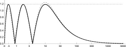
Approximation 1: $R(t)=1+t+t^2/(at+b)$, $a=1.991162$, $b=10.05113$, . Rounding $a$ to 2 and $b$ to 10 increases the maximum absolute error to $1.25\times {10}^{-3}$, but also reduces the absolute errors over a substantial interval. The maximum absolute error of Winitzki’s approximation (one parameter) is $2.76\times {10}^{-2}$, after converting it from erf to normal and optimizing the parameter. The maximum absolute error of Hastings’ sheet 67 (four parameters) is $2.84\times {10}^{-3}$.

Unlike many approximations, there is little to be gained by optimizing approximation 1 over a domain that excludes very small values of $q$. On the other hand, increasing the degree of $R$ provides a substantial gain in accuracy without restricting $q$.

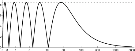
Approximation 2: $R(t)=1+t+t^2(at+b)/(t^2+ct+d)$, $a=.5583971$, $b=6.268748$, $c=20.36848$, $d=58.95569$, .

The maximum absolute error of Hastings’ sheet 68 (six parameters) is $4.47\times {10}^{-4}$. The maximum absolute error of the Hill–Davis approximation (six parameters) is $3.58\times {10}^{-4}$ if $|z|\le 304$; otherwise the limit is $7.11\times {10}^{-4}$.

Fig. 1 and Fig. 2 show the absolute error curves for approximations 1 and 2. The dashed curve in Fig. 1 shows the result of rounding $a$ and $b$ to integers. To display the asymptotic behavior of the approximations, the $z$ axis in all the figures extends far beyond the usual single-digit range and is plotted in arcsinh units. The computations used Mathematica’s arbitrary precision capability.

Figure 1. Approximation 1: ${10}^3|\widehat{z}-z|$ as a function of $z$. Optimized parameters give the solid curve. Rounded parameters give the dashed curve.

Figure 2. Approximation 2: ${10}^5|\widehat{z}-z|$ as a function of $z$.

Simple approximations are no longer as widely needed as they once were, but where simplicity is still important, approximation 1 is so simple, especially with the rounded parameters, that it should be used if its error bound is acceptable; if it is not, then approximation 2 should be considered. No other approximations of comparable simplicity have such small absolute errors over the full range of $z$.

Aside from any immediate practical uses these approximations may have, the fact that they are so simple, yet still manage to cover the full range with smaller errors than many more complex approximations, suggests that further study is warranted to see why they are so much better than the others and how far that advantage extends. Investigating the general form of the approximation ${(t-\ln R(t))}^{1/2}$, with $R$ not necessarily a rational function, would accordingly be a logical next step, consonant with Howard’s (2022) [8] suggestion “that finding approximations to the inverse error function is best treated directly and as a separate problem, rather than approaching it via finding the inverse of an approximation to the error function.”

3. A Different Approach

It may not always be appropriate to minimize the absolute error in $\widehat{z}$. In general, the choice of a minimand ought to be based on the intended use of the approximate value and the effects that errors in it may have. For instance, if we were constructing a table of approximate critical values $\widehat{z}$ for given values of $q$, and if each implied $\tilde{q}=\overline{F}(\widehat{z})$ would be taken as if it were the given $q$, then it might be better to minimize the relative error in $\tilde{q}$ rather than the absolute error in $\widehat{z}$. This approach — comparing $\tilde{q}$ to the original $q$ — is analogous to evaluating a translation from one language to another by comparing its back-translation to the original. It seems to have not been used before to evaluate numeric approximations.

Alternate approximation 1: $a=1.80977$, $b=11.627$, .

Alternate approximation 2: $a=.5688184$, $b=14.97873$, $c=38.46443$, $d=145.668$, .

Figure 3. Alternate approximation 1: ${10}^3|\ln (\tilde{q}/q)|$ as a function of $z$.

Figure 4. Alternate approximation 2: ${10}^4|\ln (\tilde{q}/q)|$ as a function of $z$.

Fig. 3 and Fig. 4 show the relative error curves for the alternate approximations. The asymptotic relative error can be made zero by setting $a$ to $2/(\pi \mathrm{–}2)$ in the first approximation or $\pi /2\mathrm{–}1$ in the second, but that would increase the maximum relative error even after adjusting the other parameters to equate the magnitudes of the extrema.

The alternate approximations, too, may have some immediate practical uses, but there is a larger point to be made here. Minimizing the relative error in $\tilde{q}$ is equivalent to minimizing the weighted error in $\widehat{z}$ using weights that increase with $z$, which is opposite to the weighting needed to minimize the relative error in $\widehat{z}$. The relative seriousness of errors in $\widehat{z}$ at different values of $z$ will depend on what $z$ represents and the effects that errors in $\widehat{z}$ will have, which is a subject-field question; there is unlikely to be one approximation that is best for all purposes. This is true for approximations in general, not just the inverse-normal.