Stability of piecewise flat Ricci flow
in three dimensions

Abstract.

For a recently developed piecewise flat approximation of the Ricci flow, numerical instabilities are seen to arise for a particularly useful class of mesh-types. Here, a geometrically motivated adaptation to these meshes is introduced, and a linear stability analysis and numerical simulations used to show that the instability is then suppressed. These adapted meshes have also been successfully used in a recently published paper to show the convergence of the piecewise flat Ricci flow to known smooth Ricci flow solutions for a variety of manifolds.

1. Introduction

The Ricci flow is a uniformizing flow on manifolds, evolving the metric to reduce the strength of the Ricci curvature. It was initially developed by Richard Hamilton to help prove the Thurston geometrization conjecture [2], and it remains an important tool for analysing the interplay between geometry and topology. Recently, its use has expanded further, with numerical evolutions finding applications in facial recognition [3], cancer detection [4], and space-time physics [5, 6, 7].

Piecewise flat manifolds, formed by joining flat Euclidean segments in a consistent manner, provide a remarkably useful approach for numerically evolving geometry. In particular, setting the piecewise flat segments to be simplices (triangles, tetrahedra, etc.) results in a notable separation of the topology, which is fixed by the graph structure, from the geometry, which is completely determined by a discrete set of edge-lengths. This conveniently leads to a piecewise flat Ricci flow as a rate of change of the edge-lengths. Since the graph determines the topology, there is also no need for additional boundary conditions, avoiding issues with coordinate singularities or transformations between coordinate charts. In other approaches, these have required careful consideration [8, 9, 10, 11], or the use of ambient coordinates from an embedding in a higher-dimensional Euclidean space [12, 13]. These advantages have led to extensive use of a piecewise flat Ricci flow in two dimensions [3, 4], and a piecewise flat approach in three-dimensions for manifolds with a high degree of symmetry [14, 15, 16].

A new three-dimensional piecewise flat approach, that does not require any symmetry restrictions, was introduced in [17] and has been shown to converge to known smooth Ricci flow solutions for a variety of different manifolds and piecewise flat approximations [17, 18, 19]. In this approach, the rate of change of edge-lengths is determined by an approximation of the smooth Ricci curvature at the edges, which is given in an easily computable combinatoric form, depending only on the edge-lengths and a choice of dual tessellation.

This paper concerns an instability that arises when a particularly useful mesh of cube-like blocks, each composed of six tetrahedra, is used with this new approach. A method for suppressing the instability is developed, using blocks that are internally flat instead of just being composed of flat tetrahdera. This is implemented by constraining the length of an edge in the interior of each block to make the interior flat, while retaining the simplicial structure of the graph. A linear stability analysis and numerical simulations are then used to demonstrate both the initial instability and the effectiveness of its suppression.

Computations using these adapted piecewise flat manifolds can already be seen in [18], where they have successfully been used in the piecewise flat Ricci flow of a variety of manifolds, from those with non-trivial topologies to manifolds with no continuous symmetries, showing convergence to known Ricci flow solutions and behaviour. This is particularly impressive, since most numerical Ricci flow computations in three dimensions have been restricted to single-parameter spherically-symmetric models [8, 9, 10, 11, 13, 15, 16].

The rest of the paper begins with an introduction to the piecewise flat manifolds used in this paper and the piecewise flat Ricci flow, summarizing the main results from [17]. The numerical instabilities are described in Section 3, along with a motivation and explanation of the suppression method. A linear stability analysis in Section 4 shows the exponential growth to arise from the numerical errors in the length measurements, with numerical simulations matching the growth rates. In Section 5, the same linear stability analysis no longer indicates an exponential growth when the suppressing method is used, with numerical simulations also showing stable behaviour.

2. Background

2.1. Piecewise flat manifolds and triangulations

In three dimensions, the most simple of piecewise flat manifolds are formed by joining Euclidean tetrahedra together, with the triangular faces between neighbouring tetrahedra identified. The resulting graph encodes the topology of the manifold, with the geometry completely determined by the set of edge-lengths. Piecewise flat approximations of smooth manifolds can be constructed by first setting up a tetrahedral graph on the smooth manifold, using geodesic segments as edges. A piecewise flat manifold can then be defined using the same graph, with the edge-lengths determined by the lengths of the corresponding geodesic segments on the smooth manifold. Such a piecewise flat approximation is known as a triangulation of the smooth manifold.

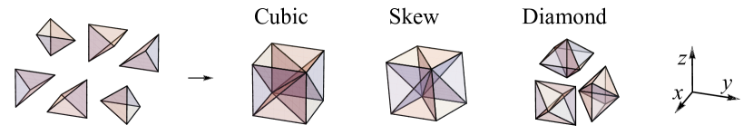
In order to test for convergence to smooth curvature and Ricci flow, a set of triangulations which can be scaled in some regular way must be used. Three such triangulation-types were defined in [18], using building blocks which can be tiled to form a complete tetrahedral graph. These building blocks are defined below, in terms of a set of coordinates $x$, $y$, and $z$, with each block covering a unit of volume. Diagrams of each block are also shown in Fig. 1.

1. The cubic block forms a coordinate cube composed of six tetrahedra, with three independent edges along the coordinate directions, three independent face-diagonals and a single internal body-diagonal. The tetrahedra are specified so that the face-diagonals on opposite sides are in the same directions.

2. The skew block has the same structure as the cubic block, but with its vertices skewed in the $x$ and $z$ directions, with $v_x=(1,-1/3,0)$ and $v_z=(-1/3,-2/9,1)$.

3. The diamond block is constructed from a set of four tetrahedra around each coordinate axis, with edges in the outer rings formed by the remaining coordinate directions.

Figure 1. The three different block types, with the six tetrahedra of the cubic block on the far left, and a slight separation of the three diamond shapes forming the diamond block.

These blocks can be used to triangulate manifolds with three-torus ($T^3$) topologies, using a cuboid-type grid of blocks to cover the fundamental domain, identifying the triangles, edges and vertices on opposite sides. The resulting triangulations have computational domains that are compact without boundary. Manifolds with other topologies can also be triangulated using these blocks but require slightly more complicated tetrahedral graphs, see for example the Nil manifold in [18]. Since the stability should depend on the local structure of the piecewise flat manifold, only $T^3$ topology triangulations will be considered here.

2.2. Piecewise flat curvature and Ricci Flow

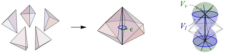
While any neighbouring pair of tetrahedra in a piecewise flat manifold still forms a Euclidean space, a natural measure of curvature arises from the sum of the dihedral angles ${\theta }_t$ around an edge $\mathrm{\ell }$, see Fig. 2, with the difference from $2\pi$ radians known as a deficit angle,

(1) $${ϵ}_{\mathrm{\ell }}:=2\pi -\sum _t{\theta }_t.$$

Triangulations of smooth manifolds are deemed good approximations if the deficit angles are uniformly small. The resolution of a piecewise flat approximation can then be increased by having a higher concentration of tetrahedra, or a finer grid of the blocks defined above.

Figure 2. The deficit angle $ϵ$ at an edge, and the edge-region $V_{\mathrm{\ell }}$ formed from the dual vertex regions $V_v$ at either end of the edge.

Conceptually, the deficit angles correspond to surface integrals of the sectional curvature orthogonal to each edge. However, a number of examples show that a single deficit angle does not carry enough information to approximate the smooth curvature directly, see Section 5.1 of [17] for example. Instead, this correspondence is used to construct volume integrals of both the scalar curvature at each vertex and the sectional curvature orthogonal to each edge, which can then be used to give the Ricci curvature along the edges.

Volumes $V_v$ associated with each vertex $v$ are defined to form a dual tessellation of the piecewise flat manifold, with barycentric duals used here, where the volume is just a quarter the sum of the volumes of the tetrahedra meeting at $v$. Edge-volumes $V_{\mathrm{\ell }}$ are then defined as a union of the volumes $V_v$ for the vertices on either end, capped by surfaces orthogonal to the edges at each vertex, as shown in Fig. 2. For the triangulations used here, this can be effectively approximated by averaging the barycentric volumes at either end of each edge. From [17], piecewise flat approximations of the scalar curvature $R_v$ at each vertex $v$, sectional curvature $K_{\mathrm{\ell }}^{⟂}$ orthogonal to each edge $\mathrm{\ell }$, and the Ricci curvature $R{c}_{\mathrm{\ell }}$ along each edge $\mathrm{\ell }$, are given by the expressions:

(2a) $R_v$ $=\frac{1}{V_v}{\displaystyle \sum _i}|{\mathrm{\ell }}_i|{ϵ}_i,$

(2b) $K_{\mathrm{\ell }}^{⟂}$ $=\frac{1}{V_{\mathrm{\ell }}}\left(|\mathrm{\ell }|{ϵ}_{\mathrm{\ell }}+{\displaystyle \sum _i}\frac{1}{2}|{\mathrm{\ell }}_i|{\cos }^2({\theta }_i){ϵ}_i\right),$

(2c) $R{c}_{\mathrm{\ell }}$ $=\frac{1}{4}(R_{v_1}+R_{v_2})-K_{\mathrm{\ell }}^{⟂},$

with the indices $i$ labelling the edges intersecting the volumes $V_v$ and $V_{\mathrm{\ell }}$, ${\theta }_i$ representing the angle between the edge ${\mathrm{\ell }}_i$ and $\mathrm{\ell }$, and $v_1$ and $v_2$ indicating the vertices bounding $\mathrm{\ell }$. Computations for a number of manifolds have shown these expressions to converge to their corresponding smooth values [17]. Similar constructions have also been developed for the extrinsic curvature [20], with numerical computations successfully converging to their smooth values.

The Ricci flow of a smooth manifold changes the metric $g$ due to the Ricci curvature $Rc$,

(3) $$\frac{dg}{dt}=-2Rc.$$

The resulting change in the length of a geodesic segment can be given solely by the Ricci curvature along and tangent to it, as shown in section 6.3 of [17]. Since the edge-lengths of a triangulation correspond to the lengths of these geodesic segments, a piecewise flat approximation of the smooth Ricci flow can be given by a fractional change in the edge-lengths,

(4) $$\frac{1}{|\mathrm{\ell }|}\frac{d|\mathrm{\ell }|}{dt}=-R{c}_{\mathrm{\ell }}$$

The equation above has been shown to converge to known smooth Ricci flow solutions as the resolution is increased, using analytic computations for symmetric manifolds in [17], and numerical evolutions for a variety of other manifolds in [18]. This approach has also been used by Alsing, Miller and Yau [19] for approximating the Ricci flow of the neckpinch model, but with a different edge volume $V_{\mathrm{\ell }}$, which works when the triangulations are adapted to the spherical symmetry of the manifolds studied there.

3. Instability and suppression

3.1. Instability

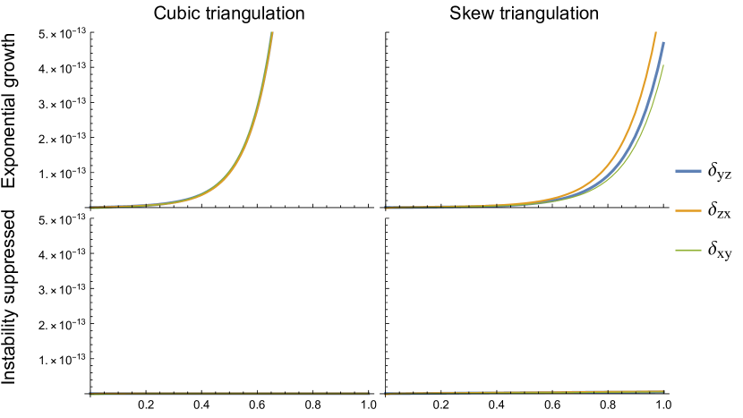
Despite the close approximation of the piecewise flat Ricci curvature $R{c}_{\mathrm{\ell }}$ to its corresponding smooth values [17], direct application of the piecewise flat Ricci flow equations to cubic and skew triangulations result in an exponential growth of the face-diagonals, even for manifolds that are initially flat. Since the deficit angles should all be zero for triangulations of a flat manifold, this growth must arise from numerical errors.

The top two graphs in Fig. 3 show how far the face-diagonal edge-lengths deviate from a flat triangulation. These deviations start at the level of the numerical precision and grow exponentially from there, soon dominating any evolution. The growth is invariant to the step size, has occurred for every grid size tested and for both the normalized and non-normalized piecewise flat Ricci flow equations. The growth rates also increase when the scale of the edge-lengths is reduced, countering any improved precision from an increase in resolution. However, these instabilities do not arise for the diamond triangulations for any of these situations. This has led to the proposition below.

Proposition 1.

The cubic and skew type triangulations lead to an exponential instability for direct application of the piecewise flat Ricci flow.

This proposition is proved in Section 4.2 using a linear stability analysis of all cubic and skew triangulations of a three-torus. Section 4.3 then shows the growth rates for a number of numerical simulations to be in close agreement with the results of the linear stability analysis.

Figure 3. Exponential growth of the errors in the face-diagonals is shown on the top row, for both cubic and skew triangulations of a flat three-torus. The bottom shows the suppression of this growth when the body-diagonals are adjusted to give blocks with flat interiors.

3.2. Suppressing instability

While it is clear that the evolution shown on the top row of Fig. 3 does not correspond to smooth Ricci flow, it is also inherently non-smooth in nature, particularly with the growth rates increasing as the resolution of a triangulation is increased. This suggests an extra freedom in the cubic and skew triangulations that does not arise in smooth manifolds.

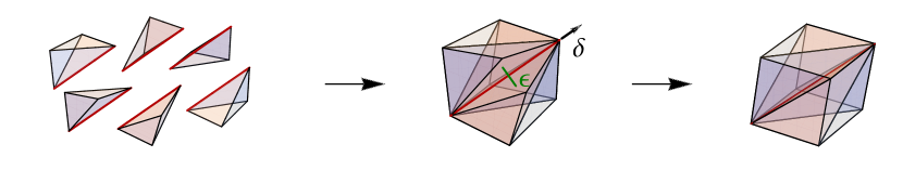
In both the linearized equations in Section 4.2, and the numerical simulations in Section 4.3, all of the face-diagonal edges can be seen to grow at the same growth rate, with the other types of edges remaining unchanged. With only the face-diagonals growing, each face can still be viewed as a flat parallelogram. The exterior of each block can also still be embedded in three dimensional Euclidean space as a parallelepiped, with the change in the face-diagonals acting similar to a change of coordinates. This is shown in the left two images of Fig. 4. The distance between the bottom left and top right vertices of the parallelepiped in the middle image of Fig. 4 must clearly grow if it is to remain embedded in Euclidean space, but the corresponding body-diagonals remain unchanged. This produces a growing deficit angle around the body-diagonals, shown on the right of Fig. 4, which then drives the growth of the face-diagonals. The addition of the body diagonal to each block can also be interpreted as producing an over-determined system, with seven edge-lengths associated with each vertex or block, while there are only six metric components at each point of a smooth manifold. However, this interpretation also suggests a solution.

Figure 4. The effect of the face-diagonal growth on the exterior of a cubic block, with the resulting deficit angle arising from an unchanged body-diagonal shown on the right.

The flat segments of a piecewise flat manifold do not necessarily have to be tetrahedra, these are just the most simple of segments. If each block of the cubic and skew triangulations are instead treated as flat, the mechanism that drives the exponential growth of the face-diagonals will be broken. This has lead to the following:

Proposition 2.

The exponential instability is suppressed for the piecewise flat Ricci flow of cubic and skew type piecewise flat manifolds with flat blocks as the piecewise flat segments.

In practice the body-diagonals are retained since it is easier to compute dihedral angles and volumes with a tetrahedral graph. Their lengths are then continually re-defined to give zero deficit angles around them, and hence a flat interior for each block, as shown in Fig. 5. This results in a set of constraint equations to determine the lengths of the body-diagonals at each step of an evolution, circumventing the over-determined nature of the tetrahedral triangulations.

Figure 5. The deficit angle $ϵ$ at the body-diagonal is shown, along with the perturbation $\delta$ of the body-diagonal that makes this deficit angle zero, giving a flat interior for the block.

Proposition 2 is proved for a number of cubic and skew grids of $T^3$ manifolds in Section 5.1, and numerical simulations show the suppression of the instability in Section 5.2. The use of flat blocks has also given stable evolutions for all of the computations in [18], giving remarkably close approximations to their corresponding smooth Ricci flows.

4. Initial instability

Since it is the linear terms in a set of differential equations that lead to exponential growth, the linear stability of the piecewise flat Ricci flow was tested for cubic and skew triangulations of flat $T^3$ manifolds.

4.1. Linear stability analysis

A linear stability analysis uses the linear terms of a perturbation away from an equilibrium to test for the stability of that equilibrium.

Definition 3.

For a system of differential equations $\frac{d{x}_i}{dt}=f_i(x_j)$:

1. A stationary solution $x_i=x_i^0$ is a solution that does not change with $t$, i.e. $\frac{d{x}_i^0}{dt}=0$.

2. Linearized equations at $x_i^0$ are the linear terms in a series expansion of $f_i(x_j^0+{\delta }_j)$ about ${\delta }_j=0$. The zero order terms vanish since they correspond to a stationary solution, resulting in the equations $\frac{d{\delta }_i}{dt}=a_{ij}{\delta }_j$ with real numbers $a_{ij}$.

3. The system is linearly unstable at $x_i^0$ if the coefficient matrix $A=a_{ij}$ for the linearized equations has any eigenvalues with positive real parts. Solutions of the linearized equations consist of linear combinations of exponential functions, with the eigenvalues of $A$ giving the growth rates.

Euclidean metrics provide stationary solutions for the smooth Ricci flow, having zero Ricci curvature, and triangulations of flat Euclidean manifolds are stationary for the piecewise flat Ricci flow, with zero deficit angles and therefore zero piecewise flat Ricci curvature. The edge-lengths for cubic and skew triangulations of flat Euclidean space, with unit volume blocks, are given in Table 1 below.

	${\mathrm{\ell }}_x$	${\mathrm{\ell }}_y$	${\mathrm{\ell }}_z$	${\mathrm{\ell }}_{yz}$	${\mathrm{\ell }}_{zx}$	${\mathrm{\ell }}_{xy}$	${\mathrm{\ell }}_{xyz}$
Cubic	$1$	$1$	$1$	$\sqrt{2}$	$\sqrt{2}$	$\sqrt{2}$	$\sqrt{3}$
Skew	$\frac{1}{3}\sqrt{10}$	$1$	$\frac{1}{9}\sqrt{94}$	$\frac{1}{9}\sqrt{139}$	$\frac{1}{9}\sqrt{142}$	$\frac{1}{3}\sqrt{13}$	$\frac{1}{9}\sqrt{133}$

Table 1. The edge-lengths for flat triangulations with unit volume blocks.

Any global scaling of the edge-lengths in Table 1 will also be stationary solutions of the piecewise flat Ricci flow. However, the linearized equations and the eigenvalues of the coefficient matrix are not invariant to this rescaling. The effect of globally rescaling the triangulation blocks is therefore given below.

Lemma 4 (Scale factor).

If a triangulation of a flat manifold has a coefficient matrix $A$, then the coefficient matrix for a rescaling of all of the edges by a factor of $c$ will be $\frac{1}{c^2}A$.

Proof.

From Eq. 2, the piecewise flat Ricci curvature for an edge ${\mathrm{\ell }}_i$ can be written as the sum

(5) $$R{c}_i=\sum _k{b}_{ik}\frac{|{\mathrm{\ell }}_k|{ϵ}_k}{V_k},$$

for some coefficients $b_{ik}$. The series expansion of $R{c}_i$ for a perturbation ${\delta }_j$ of some edge ${\mathrm{\ell }}_j$ is given by the series expansions of the individual terms appearing on the right-hand side above. The zero-order terms for the deficit angles ${ϵ}_k$ will always be zero, since these correspond to a triangulation of Euclidean space. Hence, the linear terms in the expansion of $R{c}_i$ must be given by the linear terms from the deficit angles, and the zero-order terms, or non-perturbed values, for the remaining variables.

For a global rescaling of all the edge-lengths of a triangulation by a factor of $c$, the volumes are clearly scaled by $c^3$. The coefficients $b_{ik}$ can be seen in Eq. 2 to be either constant or depend on the angles between edges, and therefore not depend on the scaling. This gives the relations

(6) $$|{\mathrm{\ell }}_k^c|=c|{\mathrm{\ell }}_k|,V_k^c=c^3{V}_k,b_{ik}^c=b_{ik},$$

with the superscript $c$ representing the rescaled terms. The deficit angles depend on the relative lengths of the edges, and since the perturbation ${\delta }_j$ is the only length that is not rescaled by $c$, the deficit angle would be the same if only ${\delta }_j$ was rescaled, but by a factor of $1/c$. An expansion of the deficit angle ${ϵ}_k^c({\delta }_j)$ for the rescaled blocks is therefore given by the equation

(7) $${ϵ}_k^c({\delta }_j)={ϵ}_{kj}^c{\delta }_j+𝒪({\delta }_j^2)=\frac{1}{c}{ϵ}_{kj}{\delta }_j+𝒪({\delta }_j^2),$$

with ${ϵ}_{kj}^c$ and ${ϵ}_{kj}$ representing the first order coefficients.

Using the piecewise flat Ricci flow equation, Eq. 4, the linear coefficients $a_{ij}^c$ for the rescaled triangulation can now be given in terms of the linear coefficient $a_{ij}$ for the original triangulation,

(8) $$a_{ij}^c=-|{\mathrm{\ell }}_i^c|\sum _k{b}_{ik}^c\frac{|{\mathrm{\ell }}_k^c|{ϵ}_{kj}^c}{V_k^c}=-\left(c|{\mathrm{\ell }}_i|\right)\sum _k{b}_{ik}\frac{\left(c|{\mathrm{\ell }}_k|\right)\left(\frac{1}{c}{ϵ}_{kj}\right)}{c^3{V}_k}=\frac{1}{c^2}{a}_{ij}.$$

The coefficient matrix $A$, and hence its eigenvalues, are therefore scaled by a factor of $1/c^2$ when all the edge-lengths of a triangulation are rescaled by $c$. ∎

4.2. Proof of Proposition 1

To calculate the linearized equations for the piecewise flat Ricci flow, a number of properties of both the graph structure and the linearization itself are taken advantage of.

• It is only necessary to determine the linearized equations for a single set of three face-diagonals due to the symmetry of the grids. The equations for all of the other face-diagonals will have the same coefficients, with an appropriate translation of indices.

• A $3\times 3\times 3$ grid of cubic or skew blocks provides all of the edges required to determine the piecewise flat Ricci curvature for the edges in the central block. This can be seen from Eq. 2, where the piecewise flat Ricci curvature $R{c}_{\mathrm{\ell }}$ depends only on the deficit angles at edges ${\mathrm{\ell }}_j$ that have a vertex in common with $\mathrm{\ell }$, and these depend only on the lengths of edges in tetrahedra containing the edge ${\mathrm{\ell }}_j$.

• Series expansions of the piecewise flat Ricci curvature need only be computed for a single perturbation variable at a time, with the linear terms for each perturbation computed separately and then added together to give the complete linearized equation. This avoids the need to compute series expansions of multiple variables simultaneously.

Symbolic manipulations in Mathematica were used to calculate the linearized equations for both the cubic and skew triangulations, with the code and results available in the Zenodo repository at https://doi.org/10.5281/zenodo.8067524.

Theorem 5 (Linear instability of cubic triangulations).

The piecewise flat Ricci flow of any cubic triangulation of a flat $T^3$ manifold is linearly unstable, with perturbations growing exponentially at a rate of at least $12/c^2$ for blocks with volume $c^3$.

Proof.

To begin, the linearized equations for the piecewise flat Ricci flow equations about a flat cubic triangulation with unit volume blocks are calculated. Each face-diagonal in a $3\times 3\times 3$ grid of cubic blocks is perturbed in turn, with the linearized equations at a set of three face-diagonals in the central block computed for each perturbation, and the contributions from all of these perturbations then added together. The resulting linearized equation at the $xy$-face-diagonal takes the form:

(9) $\frac{d}{dt}$ ${\delta }_{xy}(0,0,0)=$

$-4{\delta }_{xy}(0,0,0)-{\delta }_{xy}(-1,-1,0)-{\delta }_{xy}(1,1,0)$

$+\frac{3}{2}\left({\delta }_{xy}(-1,0,0)+{\delta }_{xy}(0,-1,0)+{\delta }_{xy}(0,1,0)+{\delta }_{xy}(1,0,0)\right)$

$+\mathrm{\hspace{0.17em}2}\left({\delta }_{xy}(0,0,-1)+{\delta }_{xy}(0,0,1)\right)$

$-\frac{1}{2}\left({\delta }_{yz}(0,-1,-1)+{\delta }_{yz}(1,1,0)\right)+{\delta }_{yz}(0,-1,0)+{\delta }_{yz}(1,1,-1)$

$+\frac{3}{2}\left({\delta }_{yz}(0,0,0)+{\delta }_{yz}(1,0,-1)\right)$

$-\frac{1}{2}\left({\delta }_{zx}(-1,0,-1)+{\delta }_{zx}(1,1,0)\right)+{\delta }_{zx}(-1,0,0)+{\delta }_{zx}(1,1,-1)$

$+\frac{3}{2}\left({\delta }_{zx}(0,0,0)+{\delta }_{zx}(0,1,-1)\right),$

with the coordinates in parentheses indicating the location of the perturbed edge in the triangulation grid, with respect to the central block. Due to the symmetries in the cubic lattice, the linearized equations for the other two face-diagonals are given by a permutation of the $\{xy,yz,zx\}$ subscripts and a similar permutation of the grid coordinates. The linearized equation for any face-diagonal in a $T^3$ grid of cubic blocks can then be given by a discrete linear transformation of the grid coordinates.

The set of coefficients in Eq. 9 are the same for the linearized equations at all of the face-diagonals in the triangulation, for any size grid, so the set of elements in each row of the coefficient matrix $A$ will also be the same. These elements sum to $12$, which must be an eigenvalue of $A$ with a corresponding eigenvector consisting of all ones. From Lemma 4, the coefficient matrix for a triangulation with blocks of volume $c^3$ will have an eigenvalue of $12/c^2$. Any solution to the set of linearized equations must then contain an exponential term with a growth rate of $12/c^2$, leading to an exponential growth for the perturbations in all of the face-diagonals of at least this rate. ∎

Theorem 6 (Linear instability of skew triangulations).

The piecewise flat Ricci flow of any skew triangulation of a flat $T^3$ manifold is linearly unstable, with perturbations growing exponentially at a rate of at least $0.996/c^2$ for blocks with volume $c^3$.

Proof.

As with the cubic triangulations in Theorem 5, the linearized equations about a flat skew triangulation with unit volume blocks are first computed. Unlike the cubic case, the skew blocks do not have the same symmetries as the cubic blocks, so the linearized equations for each of the three types of face-diagonals, ${\mathrm{\ell }}_{xy}$, ${\mathrm{\ell }}_{yz}$ and ${\mathrm{\ell }}_{zx}$ must be found separately. The linearized equations are not displayed here, but can be found in the Zenodo repository, https://doi.org/10.5281/zenodo.8067524. As with the cubic case, the linearized equations for all of the face-diagonals in a $T^3$ grid of skew blocks can be given by a discrete transformation of the grid coordinates for each of the three face-diagonals in a single block.

From these equations, it can be seen that the sum of the coefficients are not the same for each face-diagonal, so the vector of all ones is not an eigenvector for the coefficient matrix $A$ as it was for the cubic triangulations. However, by ordering the indices of the face-diagonals ${\mathrm{\ell }}_i$ according to their edge-type, a similar approach can be used. The indices for an $n$-block triangulation are defined so that $i\in \{1,\mathrm{\dots },n\}$ for the $yz$-diagonals, $i\in \{n+1,\mathrm{\dots },2n\}$ for the $zx$-diagonals and $i\in \{2n+1,\mathrm{\dots },3n\}$ for the $xy$-diagonals. Defining a vector $v$ so that

(10)

the product of the matrix $A$ with $v$ is

(11) $$A\cdot v=a_{ij}\cdot v_j=\left(\sum _{j=1}^n{a}_{ij}\right)p+\left(\sum _{j=n+1}^{2n}{a}_{ij}\right)q+\left(\sum _{j=2n+1}^{3n}{a}_{ij}\right)r.$$

Since there will only be three different values for the elements of the resulting vector, one for each type of face-diagonal, the information in this product can be reduced to the $3\times 3$ matrix product below,

(12)

with the matrix elements obtained by summing the appropriate coefficients in the linearized equations. This matrix has a maximum eigenvalue of approximately $0.966$, with a corresponding eigenvector of $(0.532,0.710,0.461)$. From Eq. 11, the matrix $A$ must also have this eigenvalue, with eigenvector $v$ from Eq. 10 where $p=0.532$, $q=0.710$ and $r=0.461$.

From Lemma 4, the coefficient matrix for a triangulation with blocks of volume $c^3$ will have an eigenvalue of approximately $0.966/c^2$. Any solution to the set of linearized equations must then contain an exponential term with a growth rate of approximately $0.966/c^2$, leading to an exponential growth for the perturbations in all of the face-diagonals of at least this rate. ∎

The linearized equations in the proofs of theorems 5 and 6 have also been used to construct the coefficient matrices for $3\times 3\times 3$ and $3\times 3\times 4$ grids of blocks using Mathematica. This was done for both the cubic and skew blocks, with the edge-lengths from Table 1, and for a rescaling of these edges by a factor of $1/3$. The eigenvalues for each matrix were then computed, again using Mathematica, with the largest real parts matching the eigenvalues in Theorem 5 and Theorem 6, as shown in Table 2.

	$c=1$		$c=1/3$
	$3\times 3\times 3$	$3\times 3\times 4$	$3\times 3\times 3$	$3\times 3\times 4$
Cubic	$12,\mathrm{\hspace{0.17em}6},\mathrm{\hspace{0.17em}2.739},\mathrm{\hspace{0.17em}0}$	$12,\mathrm{\hspace{0.17em}8},\mathrm{\hspace{0.17em}6},\mathrm{\hspace{0.17em}4.514}$	$108,\mathrm{\hspace{0.17em}54},\mathrm{\hspace{0.17em}24.65},\mathrm{\hspace{0.17em}0}$	$108,\mathrm{\hspace{0.17em}72},\mathrm{\hspace{0.17em}54},\mathrm{\hspace{0.17em}40.63}$
Skew	$0.966,0.$	$0.966,0.$	$8.697,0.$	$8.697,0.$

Table 2. The largest of the real parts of the eigenvalues for both cubic and skew triangulations, with two different grid sizes and two different scales $c$. The non-integer values are approximated to three decimal places.

Remark 7.

Due to the effect of the scaling factor $c$ in Lemma 4, the instabilities are more severe when the grid resolutions are increased. This is the opposite of the piecewise flat approximations, which should converge to their corresponding smooth values as the resolution is increased.

Remark 8.

The instability for the skew triangulations is an order of magnitude less than for the cubic triangulations for the same block volumes. It can also be noted that the cubic blocks are only borderline Delaunay for a flat manifold, with the circumcentres of all tetrahedra in a single block coinciding at the centre of that block. The skew blocks were initially used because they form more strongly Delauney triangulations, where Voronoi dual volumes can be used with more confidence. For a flat diamond block, the circumcentres of all of the tetrahedra coincide with their barycentres, making them as strongly Delaunay as possible, and may offer a clue to explain the original lack of instability in the diamond triangulations.

4.3. Numerical simulations

Simulations have been run for the piecewise flat Ricci flow of $3\times 3\times 3$, $4\times 4\times 4$ and $5\times 5\times 5$ grids of both cubic and skew blocks. The base edge-lengths were taken from Table 1, scaled by a factor of $1/3$ for the skew triangulations, with Theorem 5 and Theorem 6 indicating that these should give exponential growth rates on the order of $10$. The edge-lengths were then approximated as double-precision floating point numbers, and each perturbed by a random number from a normal distribution with standard deviation of ${10}^{-15}$, the level of numerical precision. Evolutions were performed using an Euler method with 100 steps of size 0.01, and deviations in the face-diagonal edge-lengths were fitted to a linear combination of exponential functions,

(13) $f_{cubic}(t)$ $=a_1{e}^{k_{1}t}+a_2{e}^{k_{2}t}+a_3{e}^{k_{3}t}+c,$

$f_{skew}(t)$ $=a_1{e}^{k_{1}t}+bt+c.$

The number of terms was chosen to include all of the positive eigenvalues for the $3\times 3\times 3$ grid triangulations shown in Table 2. A linear term was also added for the skew function, as the non-face-diagonal edges showed a consistent linear growth of about ${10}^{-15}$. Results of the growth rates and coefficient of determination ($R^2$) values for the best-fit functions are presented in Table 3, with sample graphs of the fitted functions and their corresponding data shown in Fig. 6.

		$3\times 3\times 3$	$3\times 3\times 3$		$4\times 4\times 4$		$5\times 5\times 5$
		Eigenvalues	Median	IQR	Median	IQR	Median	IQR
Cubic	$k_1$	$12$	$11.998$	$0.001$	$11.997$	$0.007$	$11.97$	$0.04$
	$k_2$	$6$	$6.04$	$0.01$	$6.04$	$0.08$	$6.2$	$0.5$
	$k_3$	$2.739$	$2.86$	$0.04$	$2.9$	$0.2$	$3.8$	$1.9$
	$R^2$		$0.99998$	${10}^{-6}$	$0.99994$	${10}^{-4}$	$0.99930$	${10}^{-3}$
Skew	$k$	$8.697$	$8.339$	$0.004$	$8.336$	$0.01$	$8.337$	$0.01$
	$R^2$		$0.999999$	${10}^{-7}$	$0.999998$	${10}^{-6}$	$0.999999$	${10}^{-6}$

Table 3. The median growth rates ($k_i$) and coefficient of determination ($R^2$) values with their interquartile ranges (IQR) for each triangulation. The values for the cubic triangulations are in extremely close agreement with the corresponding eigenvalues for the $3\times 3\times 3$ grid in Table 2 (reproduced in “Eigenvalues” column), and the skew parameters in close agreement.

Figure 6. The best-fit graphs with the lowest $R^2$ values ($0.99998$ and $0.999999$ respectively) for deviations in the edge-lengths of the $3\times 3\times 3$ grid triangulations, closely agreeing with the evolution values represented by the points.

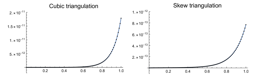
The close agreement between the growth rates in Table 3 and eigenvalues in Table 2, along with the extremely high $R^2$ values, demonstrate how effective the linearized equations are in approximating the evolution. The low interquartile ranges also show consistent behaviour across all edges, with surprisingly comparable growth rates over the different grid sizes, considering a higher number of distinct eigenvalues should be expected for larger grids. In particular, the simulations support the hypothesis that the eigenvalues in Theorem 5 and Theorem 6 represent the largest growth rates for any cubic or skew type triangulations.

5. Suppression of Exponential Instability

With the body-diagonals re-defined to give flat interiors for each block, the linear stability analysis and numerical simulations are performed again, with the exponential growth suppressed in both.

5.1. Linear instability suppressed

The linearized equations are calculated here by taking advantage of the same properties outlined at the beginning of Section 4.2, but with some additional steps to ensure that each block is flat after any perturbations.

• Once a face-diagonal ${\mathrm{\ell }}_j$ is perturbed by an arbitrary amount ${\delta }_j$, only the blocks on either side of that face are affected. For the body-diagonals of each of these blocks, the deficit angle can be found in terms of ${\delta }_j$ and the length $b$ of the body-diagonal itself.

• Setting the deficit angle to zero, the length $b$ which gives a flat block can be found in terms of ${\delta }_j$. Since only linear terms in ${\delta }_j$ will impact the linearized equations, $b$ need only be found as a linear approximation in ${\delta }_j$.

• A grid of size $4\times 4\times 4$ is now required to determine the piecewise flat Ricci flow for the edges in a central block, due to the changes in body-diagonals.

The linearized equations are first used to show that the approaches in Theorem 5 and Theorem 6 no longer imply a linear instability once flat blocks are used, and then to show that the linear instability is actually suppressed for a number of different grid sizes.

Theorem 9.

When the body-diagonals are re-defined to give flat blocks, summing rows of the linear coefficient matrix no longer implies a linear instability of the piecewise flat Ricci flow.

Proof.

Each face-diagonal ${\mathrm{\ell }}_j$ in a $4\times 4\times 4$ grid of blocks is perturbed away from the flat values in Table 1 by an arbitrary amount ${\delta }_j$, with the body-diagonals on either side of that face re-defined in terms of ${\delta }_j$ to give a zero deficit angle. The linear impact of each perturbation ${\delta }_j$ on a face-diagonal ${\mathrm{\ell }}_i$ in a central block can then be calculated using the piecewise flat Ricci flow equations, Eq. 4, and the separate terms summed to give the linearized equation for ${\mathrm{\ell }}_i$.

The resulting equation is shown below for an $xy$-face-diagonal of the cubic triangulation, with the coordinates indicating the relative locations of the face-diagonals on the grid,

(14) $\frac{d}{dt}$ ${\delta }_{xy}(0,0,0)=$

$-5{\delta }_{xy}(0,0,0)-{\delta }_{xy}(-1,-1,0)-{\delta }_{xy}(1,1,0)$

$-1/4\left({\delta }_{xy}(-1,0,1)+{\delta }_{xy}(0,-1,1)+{\delta }_{xy}(0,1,-1)+{\delta }_{xy}(1,0,-1)\right)$

$+5/4\left({\delta }_{xy}(-1,0,0)+{\delta }_{xy}(0,-1,0)+{\delta }_{xy}(0,1,0)+{\delta }_{xy}(1,0,0)\right)$

$+3/2\left({\delta }_{xy}(0,0,-1)+{\delta }_{xy}(0,0,1)\right)$

$-1/2\left({\delta }_{yz}(0,-1,-1)+{\delta }_{yz}(0,0,-1)+{\delta }_{yz}(1,0,0)+{\delta }_{yz}(1,1,0)\right)$

$-1/4\left({\delta }_{yz}(-1,0,0)+{\delta }_{yz}(0,1,-1)+{\delta }_{yz}(1,-1,0)+{\delta }_{yz}(2,0,-1)\right)$

$+3/4\left({\delta }_{yz}(0,-1,0)+{\delta }_{yz}(0,0,0)+{\delta }_{yz}(1,0,-1)+{\delta }_{yz}(1,1,-1)\right)$

$-1/2\left({\delta }_{zx}(-1,0,-1)+{\delta }_{zx}(0,0,-1)+{\delta }_{zx}(0,1,0)+{\delta }_{zx}(1,1,0)\right)$

$-1/4\left({\delta }_{zx}(-1,1,0)+{\delta }_{zx}(0,-1,0)+{\delta }_{zx}(0,2,-1)+{\delta }_{zx}(1,0,-1)\right)$

$+3/4\left({\delta }_{zx}(-1,0,0)+{\delta }_{zx}(0,0,0)+{\delta }_{zx}(0,1,-1)+{\delta }_{zx}(1,1,-1)\right).$

As in the proof of Theorem 5, the linearized equations for the other two types of face-diagonal in the cubic triangulation are simply given by a permutation of the $\{xy,yz,zx\}$ subscripts and of the grid coordinates. The linearized equations for a skew triangulation are not displayed here, but can be found in the Zenodo repository at https://doi.org/10.5281/zenodo.8067524. The linearized equations for all of the face-diagonals in any $T^3$ grid of cubic or skew blocks can be found through a discrete transformation of the grid coordinates.

The coefficients in Eq. 14 can be seen to sum to zero, with the coefficients of the linearized equations for the face-diagonals in the skew triangulation also summing to zero. This implies that the vector of all ones is an eigenvector of the coefficient matrix $A$, with an eigenvalue of zero, for all grid-sizes of both the cubic and skew triangulations. While this approach gave positive eigenvalues in Theorem 5 and Theorem 6, proving the equations there to be linearly unstable, it does not do so when flat blocks are used instead of just flat tetrahedra. ∎

Remark 10.

For many constant row-sum matrices, the eigenvalue given by the row-sum can be proved to be the largest eigenvalue. For example, if all of the coefficients except the first in Eq. 14 were positive, the Gershgorin circle theorem would be sufficient to prove this. Recent progress has also been made on eigenvalue bounds for more general constant row-sum matrices [21, 22]. Unfortunately, a proof that the same is true in this case has not been found, but direct computation of the eigenvalues below and the numerical simulations in Section 5.2 suggest that it is true.

For particular grid sizes, the linearized equations were used to construct the coefficient matrices directly, using the mathematical software Mathematica, and the set of eigenvalues computed for each. The eigenvalue with the largest real part is given for each piecewise flat manifold in Table 4. For the cubic blocks these were computed exactly, but numerical methods were required to compute the eigenvalues for the skew blocks.

	$c=1$		$c=1/3$
	$3\times 3\times 3$	$3\times 3\times 4$	$3\times 3\times 3$	$3\times 3\times 4$
Cubic	$0$	$0$	$0$	$0$
Skew	$3.0\times {10}^{-15}$	$3.3\times {10}^{-15}$	$2.0\times {10}^{-14}$	$3.7\times {10}^{-14}$

Table 4. The eigenvalues with the largest real part, showing a suppression of the linear instability when flat blocks are used.

Clearly, there cannot be any exponential growth terms for the linearized equations in the cubic triangulations since the largest real part of the eigenvalues is zero. The largest values for the skew triangulations are practically zero, being equivalent to zero for the numerical precision of the computations. While an eigenvalue of zero does not imply complete stability, it is consistent with the linearization of the smooth Ricci flow near a flat manifold, which also contains zero eigenvalues [23]. Also, since the piecewise flat curvatures depend on local regions of a piecewise flat manifold, it is deemed unlikely that the instability would re-emerge in larger grids.

5.2. Numerical simulations with instability suppressed

Numerical simulations of the piecewise flat Ricci flow have also been run with blocks that are effectively flat. In order to compare with the simulations in Section 4.3, the same triangulations and edge-length perturbations were used, and evolved using the same Euler method with 100 steps of size 0.01, but with the body-diagonal edge-lengths adapted at the beginning of each step. This was done by first adding a perturbation variable ${\delta }_j$ to the length of each body-diagonal ${\mathrm{\ell }}_j$, computing the deficit angle around ${\mathrm{\ell }}_j$ as a function of ${\delta }_j$, and then setting this equal to zero and solving for ${\delta }_j$. Since the deficit angles should already be small for a good triangulation, a linear approximation in ${\delta }_j$ about zero is used for the deficit angle, giving a unique solution for ${\delta }_j$ when set equal to zero. To show that the exponential growth is suppressed, the median and maximum changes in edge-lengths for all triangulations are shown in Table 5, with the deviations of the edge-lengths for the blocks with the largest changes shown in Fig. 7. These same edges were used for the graphs in Fig. 3.

		$3\times 3\times 3$	$4\times 4\times 4$	$5\times 5\times 5$
Cubic	Median change	$0$	$0$	$0$
	Max. change	$1.7\times {10}^{-15}$	$3.1\times {10}^{-15}$	$2.2\times {10}^{-15}$
	Initial pert.	$2.4\times {10}^{-15}$	$3.1\times {10}^{-15}$	$3.3\times {10}^{-15}$
Skew	Median change	$4.6\times {10}^{-15}$	$4.6\times {10}^{-15}$	$4.6\times {10}^{-15}$
	Max. change	$6.7\times {10}^{-15}$	$8.0\times {10}^{-15}$	$8.1\times {10}^{-15}$
	Initial pert.	$2.9\times {10}^{-15}$	$3.1\times {10}^{-15}$	$4.0\times {10}^{-15}$
	Median slope	$4.5\times {10}^{-15}$	$4.6\times {10}^{-15}$	$4.5\times {10}^{-15}$
	IQR of slope	$7.5\times {10}^{-16}$	$7.8\times {10}^{-16}$	$7.6\times {10}^{-16}$

Table 5. The median and maximum edge-length changes for each triangulation, along with the maximum values of the initial random perturbations. The median and interquartile ranges (IQR) for the best-fit linear functions in the skew triangulations are also shown. All values are close to the numerical precision, showing a suppression of the exponential growth.

Figure 7. Deviations of the face-diagonal edge-lengths from their pre-perturbed values, for blocks with the largest edge-length changes, and the corresponding rates of change from the adapted piecewise flat Ricci flow, showing a clear suppression of the exponential instability.

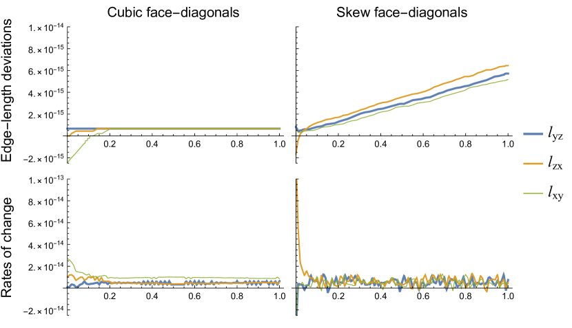
The adapting of the body-diagonals has clearly suppressed the exponential growth for both the cubic and skew simulations. For the cubic triangulations, most of the edge-lengths do not change, and those that do, only change during the first quarter of time steps and by an extremely small amount, less than the largest of the initial perturbations. While the growth rates are non-zero throughout the simulation, as seen in Fig. 7, when combined with the step size for the Euler method the resulting changes are lower than the numerical precision. The set of edge-lengths then become stationary once the rates of change drop below this threshold.

For the skew triangulations, the numerical precision is lower as it depends on the lengths of the edges, so the oscillations in the lower-right graph in Fig. 7 continue to produce a linear growth. Linear functions have therefore been fitted to the data for each edge in the triangulation, with the results in Table 5 showing consistent, extremely small rates of change across all edges, also agreeing with the rates of the background linear growth for the un-suppressed simulations in Section 4.3. While this linear growth does not directly correspond to smooth Ricci flow, it does not conflict with it either. The consistency of the rates of change lead to a global change in the scale but will not produce any curvature, so the piecewise flat manifold remains in a stationary state, growing but remaining flat. The low rate means the effect will not be noticeable at regular scales for extremely long time frames, but the effect can still be avoided by using the normalized Ricci flow which preserves the global volume.

6. Conclusion

The cubic and skew type triangulations have been successfully adapted to avoid a numerical instability resulting from the direct application of the piecewise flat Ricci flow to these triangulation types. The instability was seen to come from an over-determination of the system, with seven distinct edge-lengths associated with each block, while there are only six metric components at each point on a smooth manifold. This is resolved by removing the body diagonals as variables, and setting the interior of each block to be flat. In practice, the tetrahedral structure is retained, with a set of constraint equations introduced for the lengths of the body-diagonals so that their deficit angles vanish at each time step, ensuring a flat interior for each block.

While the instability first appeared in numerical simulations, a linear stability analysis for cubic and skew triangulations of a flat Euclidean space has indicated the same growth rates for the errors in the face diagonals. The largest growth rates were found by summing the rows of the linear coefficient matrices, and once the triangulations have been adapted, these row-sums are all zero. As with related matrices, it seems reasonable to expect the constant row-sums to give the largest real eigenvalue for each linear coefficient matrix, and hence the largest growth rates for the system. Direct computations of the largest growth rates for a number of specific grids also give zero, in agreement with the smooth Ricci flow [23], and the numerical simulations lead to stable evolutions for the adapted triangulations.

Although this paper only shows the stability for adapted triangulations of flat Euclidean manifolds, these adaptations have also led to stable piecewise flat Ricci flow for a variety of different manifolds in [18], where they were shown to converge to their expected smooth Ricci flow solutions. Also, despite re-defining the body-diagonals to have zero deficit angles, computations of the piecewise flat Ricci curvature in [18] are just as accurate at these body-diagonals as they are at the other edges, showing the robustness of the piecewise flat curvature expressions in Eq. 2.

Data Availability.

The Mathematica notebooks used for the computations and numerical simulations, and the data generated by these, are available in the Zenodo repository at https://doi.org/10.5281/zenodo.8067524.

Acknowledgements.

I would like to thank Robert Sheehan and Chris Mitchell for many helpful discussions which greatly benefited this work.