Efficient global optimization of multivariate functions with unknown Hölder constants via $\alpha$-dense curves

Abstract.

In this paper, we consider the global optimization problem of non-smooth functions over an $n$-dimensional box, satisfying the Hölder condition. We focus our study on the case when the Hölder constant is not a priori known. We develop and analyze two algorithms. The first one is an extension version of the Piyavskii’s method that adaptively construct a linear secants of the Hölder support functions, avoiding the need for a known Hölder constant. The second algorithm employs a reducing transformation approach which consists of generating, in the feasible box, an $\alpha$-dense curves, effectively converting the multivariate initial problem to a problem of a single variable. We prove the convergence of both algorithms. Their practical efficiency is evaluated through numerical experiments on some test functions and comparison with existing techniques.

1. Introduction

Let us consider the following box constrained global optimization problem of finding at least one point $x^{\ast }\in D$ and the corresponding optimal value $g^{\ast }$ such that:

(1) $$g^{\ast }=g(x^{\ast })=\underset{x\in D}{\min }g(x)$$

where the objective function $g:D\to ℝ$ is non-smooth non convex. It is assumed to satisfy the Hölder condition on the $n$-dimensional compact box $D$:

$$D=[a_1,b_1]\times \mathrm{\cdots }\times [a_n,b_n]\subset {ℝ}^n.$$

Specifically, there exist a Hölder constant $h_g>0$ and a Hölder exponent $1/\beta (\beta >1)$ such that:

(2) $$|g(x)-g(y)|\le h_g\parallel x-y\parallel {}^{1/\beta },\text{for all }x,y\in D.$$

Here, $\parallel \cdot \parallel$ denotes the Euclidean norm. A primary focus of this work is when the Hölder constant $h_g$ is not known a priori.

Many real-world optimization problems are complex, involve minimizing continuous functions of $n$ variables possessing multiple extrema over the feasible domain. Frequently, derivative information is either unavailable or its computation is expensive, rendering standard non-linear programming methods ineffective for finding global optima, as they typically converge only to local minima. Global optimization has thus become an active field of research [11]. The challenges are often amplified by local irregularities (non-smoothness) and the potential existence of numerous local minima within the feasible set. Deterministic global optimization strategies, particularly covering methods, offer a rigorous approach to tackle such problems [11, 19]. The first work on covering methods for univariate Lipschitz functions (the case $\beta =1$ in (2)) was performed by Piyavskii [13], Evtushenko [6], and Shubert [17]. The widely discussed Piyavskii-Shubert algorithm guarantees convergence to the global minimum by constructing a sequence of improving piecewise lower-bounding functions (sub-estimators) based on the known Lipschitz constant [11]. More recently, research has addressed the optimization of less regular functions satisfying the Hölder condition with $\beta >1$ [7, 12]. Gourdin et al. were among the first to study the global optimization of both univariate and multivariate Hölder functions using such deterministic approaches [7, 10].

The aim of this paper is twofold. First, we develop a novel technique for univariate Hölder optimization ($n=1$), extending the ideas of Piyavskii. This method utilizes the secants linked to the Hölder support functions between evaluated points. We address both the case where the Hölder constant $h_g$ is known and significantly, the case where the constant $h_g$ is unknown. For the latter, we propose an adaptive estimation scheme for $h_g$, which is crucial for practical application and performance. Second, we address the multivariate case ($n>1$). Direct generalization of Piyavskii’s algorithm to higher dimensions is computationally challenging, primarily because finding the minimum of the multivariate sub-estimator involves determining intersections of complex hypersurfaces [7, 20]. To overcome this, we propose an approach based on dimension reduction. This method transforms the original $n$-dimensional problem (1) into a one-dimensional Hölder optimization problems by exploring the box $D$ along an $\alpha$-dense curve [22, 23, 24]. The univariate algorithm developed in the first part can then be effectively applied to these simpler problems.

The paper is organized as follows. Section 2 presents the univariate algorithm based on Hölder support functions and secant information. Section 3 describes the reducing transformation method for the multivariate case, detailing the use of a specific $\alpha$-dense curve. Section 4 provides numerical results from experiments on test functions and compares the performance with existing methods. Section 5 concludes the work.

2. Univariate Hölder global optimization

Let us begin by considering the problem (1), (2) for a function $f$ with a single variable, i.e.,

(3) $$\underset{x\in [a,b]}{\min }f(x),a,b\in ℝ$$

where the objective function $f$ satisfying the following Hölder condition

(4) $$\left|f(x)-f(y)\right|\le h_f{\left|x-y\right|}^{1/\beta },\text{ for all}x,y\in [a,b].$$

with a constant $h_f>0$ and $\beta >1$. Let $\epsilon >0$ be the desired accuracy with which the global minimum to be searched.

2.1. Sub-estimator function

When minimizing a non-convex function $f$ over a feasible set, the general principle behind most deterministic global optimization methods is to relax the original non-convex problem in order to make the relaxed problem convex by utilizing a sub-estimator of the objective function $f$. The Hölder condition (4) allows one to construct such a lower bound for $f$ over an interval $[a,b]$. From (4) we have

$$f(y)-h_f{\left|x-y\right|}^{1/\beta }\le f(x),\forall x,y\in [a,b].$$

Let $x_{i-1}$ and $x_i$ be two distinct points in [a,b], typically with . We define the following functions:

By construction setting $y=x_{i-1}$ or $y=x_i$ in the Hölder inequality, these functions are lower bounds for $f(x)$ on their respective domains of definition within $[a,b]$:

The functions $U_{i-1}$ and $U_i$ are thus sub-estimators of $f$. Over any sub-interval $[x_{i-1},x_i]\subseteq [a,b]$, both functions are well-defined lower bounds. We can then define a tighter sub-estimator ${\psi }_i(x)$ on this sub-interval:

$${\psi }_i(x)=\max \{U_{i-1}(x),U_i(x)\}.$$

This function ${\psi }_i(x)$ is convex (as the maximum of two concave functions, assuming $1/\beta \le 1$) and non-differentiable (typically at the point where $U_{i-1}(x)=U_i(x)$). It also satisfies:

(5) $${\psi }_i(x)\le f(x),\forall x\in [x_{i-1},x_i],$$

The global minimum of ${\psi }_i(x)$ over $[x_{i-1},x_i]$ occurs at the point $\overline{x}$ where $U_{i-1}$ and $U_i(x)$ intersect (assuming such an intersection exists within the interval). This point $\overline{x}$ is given by:

$$\overline{x}=\underset{[x_{i-1},x_i]}{\arg \min }{\psi }_i(x).$$

Thus, in each iteration of Piyavskii’s algorithm, we must solve the following non-linear equation to find this intersection point:

(6) $$U_{i-1}\left(x\right)-U_i\left(x\right)=0.$$

Determining the unique solution $\overline{x}$ to equation (6) within $[x_{i-1},x_i]$ is generally straightforward only for specific values of $\beta$. For instance, Gourdin et al. [7] provide analytical expressions for this solution when $\beta \in \{2,3,4\}$, assuming $h_f$ is known a priori. However, when $\beta$ is large or not an integer, solving equation (6) can be as complex as a general non-linear local optimization problem. To overcome this difficulty, we propose a new procedure below.

2.2. Procedure approach to the intersection point

Let ${\theta }_i$ be the same midpoint of the intervals $[U_i(x_{i-1}),U_{i-1}(x_{i-1})]$ and $[U_{i-1}(x_i),U_i(x_i)]$ so

(7) $${\theta }_i=\frac{f(x_{i-1})+f(x_i)-h_f{(x_i-x_{i-1})}^{1/\beta }}{2}.$$

As $U_{i-1}(x)$ and $U_i(x)$ are monotone continuous functions on the interval $[x_{i-1},x_i]$ then they are bijective functions. Let $U_{i-1}^{-1}$ and $U_i^{-1}$ be the inverse functions respectively of $U_{i-1}$ and $U_i$. We denote by ${\mu }_i=U_{i-1}^{-1}({\theta }_i)$ and ${\vartheta }_i=U_i^{-1}({\theta }_i)$. According to the definition of $U_{i-1}$ and $U_i$ we have:

(8) $$\{\begin{array}{cc}{\mu }_i=x_{i-1}+{(\frac{f(x_{i-1})-{\theta }_i}{h_f})}^{\beta },\hfill & \\ {\vartheta }_i=x_i-{(\frac{f(x_i)-{\theta }_i}{h_f})}^{\beta }.\hfill & \end{array}$$

Let $S^{-}(x)$ and $S^{+}(x)$ be the two straight secants linked to the parables $U_{i-1}$ and $U_i$ on the interval $[{\mu }_i,{\vartheta }_i]\subset [x_{i-1},x_i]$ and joining respectively the points $({\mu }_i,{\theta }_i)$, $({\vartheta }_i,U_{i-1}({\vartheta }_i))$ and $({\mu }_i,U_i({\mu }_i))$, $({\vartheta }_i,{\theta }_i)$, we get

$$S^{-}(x)=f(x_{i-1})-h{({\vartheta }_i-x_{i-1})}^{1/\beta }+\frac{h{({\mu }_i-x_{i-1})}^{1/\beta }-h{({\vartheta }_i-x_{i-1})}^{1/\beta }}{{\vartheta }_i-{\mu }_i}(x-{\vartheta }_i),$$

$$S^{+}(x)=f(x_i)-h{(x_i-{\vartheta }_i)}^{1/\beta }+\frac{h{(x_i-{\mu }_i)}^{1/\beta }-h{(x_i-{\vartheta }_i)}^{1/\beta }}{{\vartheta }_i-{\mu }_i}(x-{\vartheta }_i).$$

The intersection point of the two secants $S^{-}$ and $S^{+}$ is the point $z_i$ the approximate point $\overline{x}$ of the two parables $U_{i-1}$ and $U_i$ (see Fig. 1).

Figure 1. Illustration of the secant-based approximation for the sub-estimator’s intersection point.

Then

(9) $$z_i=\frac{\left[f(x_{i-1})-f(x_i)-h_f{({\vartheta }_i-x_{i-1})}^{1/\beta }+h_f{(x_i-{\vartheta }_i)}^{1/\beta }\right]({\vartheta }_i-{\mu }_i)}{h_f\left[{(x_i-{\mu }_i)}^{1/\beta }-{({\mu }_i-x_{i-1})}^{1/\beta }-{(x_i-{\vartheta }_i)}^{1/\beta }+{({\vartheta }_i-x_{i-1})}^{1/\beta }\right]}+v_i.$$

Remark 1.

If $f(x_{i-1})=f(x_i)$, the approximate point $\overline{x}$ is immediately the midpoint of the interval $[x_{i-1},x_i]$. In this case, one can choose:

(10) $$z_i=\overline{x}=\frac{x_{i-1}+x_i}{2}.$$

Proposition 2.

Let $f$ be a real univariate Hölder function with the constant $h_f>0$ and $\beta >1$ defined on the interval $[a,b]$. Let the value ${𝐌}_i=\min \{U_{i-1}\left(z_i\right),U_i\left(z_i\right)\}$ (as a constant lower bound of $f$ on $[x_{i-1},x_i]\subset [a,b]$). Then we have:

(11)

Proof.

The value ${𝐌}_i$ is given by replacing the variable $x$ in the two functions $U_{i-1}\left(x\right)$ and $U_i\left(x\right)$ by the expression of $z_i$. Since we have defined the function

$${\psi }_i(x)=\max \{U_{i-1}(x),U_i(x)\},$$

as a sub-estimator function of $f(x)$ over the interval $[x_{i-1},x_i]$. Then,

$${\psi }_i(x)\le f(x),\forall x\in [x_{i-1},x_i].$$

The function $U_{i-1}(x)$ is strictly decreasing and $U_i(x)$ is strictly increasing over the interval $[x_{i-1},x_i].$ Thus, it follows

$$\min \{U_{i-1}(x),U_i(x)\}\le \underset{[x_{i-1},x_i]}{\min }{\psi }_i(x),\forall x\in [x_{i-1},x_i].$$

In particular, for $x=z_i$ it then follows:

∎

Algorithm 1 MSPA with known value of $h_f$

1:Step 1: Initialization

2:$[a,b]\subset ℝ$ a given search, Hölder parameters $h_f,\beta >1$,

3:$\epsilon$ accuracy of global minimization

4:$k\leftarrow 2,x_1\leftarrow a,x_2\leftarrow b$

5:Step k: The sampling points $x_1,x_2,\mathrm{\dots },x_k$ are ordered such that

6:for $i=2$ to $k$ do

7:  if $f(x_{i-1})\ne f(x_i)$ then

8:   ${\theta }_i$ as defined in (7), ${\mu }_i,{\vartheta }_i$ as defined in (8), $z_i$ as defined in (9)

9:  else

10:   $z_i=\frac{x_{i-1}+x_i}{2}$

11:  end if$\mathrm{𝐞𝐧𝐝}\mathrm{𝐢𝐟}$

12:  ${𝐌}_i=\min \{f(x_{i-1})-h_f{(z_i-x_{i-1})}^{1/\beta },f(x_i)-h_f{(x_i-z_i)}^{1/\beta }\}$

13:end for$\mathrm{𝐞𝐧𝐝}\mathrm{𝐟𝐨𝐫}$

14:

(12) $${𝐌}_{\rho }=\min \left\{{𝐌}_i:2\le i\le k\right\}$$

15:$z_{\rho }=\arg min\left\{{𝐌}_{\rho }\right\}$

16:$x_{\rho }=z_{\rho }$

17:if $\left|x_{\rho }-x_{\rho -1}\right|>\epsilon$ then

18:  

(13) $$x_{k+1}=z_{\rho }$$

19:  $k\leftarrow k+1$

20:  go to the Step $k$

21:else

22:  $f_{opt}=\min \left\{f(x_i):1\le i\le k\right\}$

23:  Stop

24:end if$\mathrm{𝐞𝐧𝐝}\mathrm{𝐢𝐟}$

25:return $f_{opt}$.

2.3. Convergence Result of MPSA

Theorem 3.

Let $f(x)$ be a real function defined on a closed interval $[a,b]$, satisfying (4) with $h_f>0$ and $\beta >1$. Let $x^{\ast }$ be a global minimizer of $f(x)$ over $[a,b]$. Then the sequence ${(x_k)}_{k\ge 1}$ generated by the MSPA algorithm converges to $x^{\ast }.$ i.e.,

$$\underset{k\to +\mathrm{\infty }}{lim}f(x_k)=f(x^{\ast })=\underset{x\in [a,b]}{\min }f(x).$$

Proof.

The proof is based on the construction of a sequence of points ${(x_k)}_{k\ge 1}$ generated by Algorithm 1, which converges to a limit point that is the global minimizer of $f$ on $[a,b]$. Let $x_1,x_2,x_3,\mathrm{\dots }$ be the sampling sequence satisfying (9), (12), (13). Let us consider that $x_m\ne x_{m^{\prime }}$ for all $m\ne m^{\prime },$ the set of the elements of the sequence ${(x_k)}_{k\ge 1}$ is then infinite and therefore has at least one limit point in $[a,b].$ Let $𝐳$ be any limit point of ${(x_k)}_{k\ge 1}$ such that $𝐳\ne a,$ $𝐳\ne b,$ then the convergence to $𝐳$ is bilateral (one can see [12]). Consider the interval $[x_{\mu -1},x_{\mu }]$ determined by (12) at the $(k+1)$-th iteration. According (9) and (13), we have that the new point $x_{k+1}$ divides the interval $[x_{\mu -1},x_{\mu }]$ into the subintervals $[x_{\mu -1},x_{k+1}]$ and $[x_{k+1},x_{\mu }]$, so we can deduce

(14) $$\max \{x_{k+1}-x_{\mu -1},x_{\mu }-x_{k+1}\}\le \left|x_{\mu }-x_{\mu -1}\right|.$$

Consider now an interval $[x_{\rho (k)-1},x_{\rho (k)}]$ which contains $𝐳$, using (9), (12), (13) and (14), we obtain:

(15) $$\underset{k\to +\mathrm{\infty }}{lim}(x_{\rho (k)-1}-x_{\rho (k)})=0.$$

In addition, the value ${𝐌}_{\rho (k)}$ that corresponds to $[x_{\rho (k)-1},x_{\rho (k)}],$ is given by

(16) $${𝐌}_{\rho (k)}=\min \{f(x_{\rho (k)-1})-h_f{(z_{\rho }-x_{\rho (k)-1})}^{1/\beta },f(x_{\rho (k)})-h_f{(x_{\rho (k)}-z_{\rho })}^{1/\beta }\},$$

where $z_{\rho }$ is obtained by replacing $i$ by $\rho$ in (9). As $𝐳\in [x_{\rho (k)-1},x_{\rho (k)}]$ and from (15) then we have

(17) $$\underset{k\to +\mathrm{\infty }}{lim}{𝐌}_{\rho (k)}=f(𝐳).$$

On the other hand, according to (11)

(18) $${𝐌}_{j(k)}\le f(x),\forall x\in [x_{j(k)-1},x_{j(k)}].$$

From (12), ${𝐌}_{\rho (k)}=\min \{{𝐌}_j,j=2,\mathrm{\dots },k\},$ then

$${𝐌}_{\rho (k)}\le {𝐌}_{j(k)},\forall x\in [x_{j(k)-1},x_{j(k)}],$$

and since $[a,b]=\underset{j=2}{\overset{𝑘}{\cup }}[x_{j(k)-1},x_{j(k)}]$ , hence

(19) $$\underset{k\to +\mathrm{\infty }}{lim}{𝐌}_{\rho (k)}\le {𝐌}_{j(k)},\forall x\in [a,b],$$

and from (18),(19) we get

$$\underset{k\to +\mathrm{\infty }}{lim}{𝐌}_{\rho (k)}\le f(x),\forall x\in [a,b].$$

Since $x^{\ast }$ is the global minimizer of $f$ over $[a,b]$

$$\underset{k\to +\mathrm{\infty }}{lim}{𝐌}_{\rho (k)}\le f(x^{\ast })\le f(𝐳),$$

thus, we have

$$0\le f(𝐳)-f(x^{\ast })\le f(𝐳)-\underset{k\to +\mathrm{\infty }}{lim}{𝐌}_{\rho (k)}=0,$$

then

$$f(𝐳)=f(x^{\ast })\text{. }$$

By the condition (4), the function $f$  must be continuous on $[a,b]$ so that

$$f(𝐳)=f(\underset{k\to +\mathrm{\infty }}{lim}{x}_k)=\underset{k\to +\mathrm{\infty }}{lim}f(x_k)=f(x^{\ast }).$$

∎

2.4. Estimating of unknown Hölder constant

The algorithm MSPA presented in the section 2 of this paper is applied to a class of Hölder continuous functions defined on the closed and bounded interval $[a,b]$ of $ℝ$ when suppose a priori knowledge of the Hölder constant $h_f>0$. However, the constant $h_f$ may be, in most situations, unknown and no procedure is available to obtain a guaranteed overestimate of it. Then, there is a need to find an approximate evaluation of a minimal value of $h_f$. The algorithm we will extend does not require a priori knowledge of the $h_f$. To over come this situation, a typical procedure is to look for an approximation of $h_f$ during the course of search ([11], [12], [21]). We consider a global estimate of $h_f$, for each iteration. Let the sampling points and the values $f(x_1),f(x_2),\mathrm{\dots },f(x_n)$ are also calculated. Let

$$h_f^i=\frac{\left|f(x_i)-f(x_{i-1})\right|}{{(x_i-x_{i-1})}^{1/\beta }},\text{for}i=2,\mathrm{\dots },k$$

and

$$h_f^k=\max \{h_f^i,i=2,\mathrm{\dots },k\}.$$

Let $\lambda >1$ be the multiplicative parameter as an input of the algorithm and $\nu$ be a small positive number. The global estimate of $h_f$ then is given by:

$${\tilde{h}}_f=\{\begin{array}{cc}\lambda h_f^k,\text{if}f(x_i)\ne f(x_{i-1}),\forall i\ge 2\hfill & \\ \lambda \nu ,\text{else}.\hfill & \end{array}$$

The condition $f(x_{i-1})\ne f(x_i)$, for all $i$, indicates that the objective function $f$ is not constant over the feasible interval $[a,b]$. Now from the definition of the global estimate ${\tilde{h}}_f$, we replace in the formulas of ${\theta }_i,{\mu }_i$ and ${\vartheta }_i$, the constant $h_f$ by ${\tilde{h}}_f$ also the point $(z_i,{𝐌}_i(z_i))$ is replaced in the structure of the algorithm MSPA by the point $(\widetilde{z_i},{𝐌}_i(\widetilde{z_i}))$ where:

(20) $$\widetilde{z_i}=\frac{\left[f(x_{i-1})-f(x_i)-{\tilde{h}}_f{({\vartheta }_i-x_{i-1})}^{1/\beta }+{\tilde{h}}_f{(x_i-{\vartheta }_i)}^{1/\beta }\right]({\vartheta }_i-{\mu }_i)}{{\tilde{h}}_f\left[{(x_i-{\mu }_i)}^{1/\beta }-{({\mu }_i-x_{i-1})}^{1/\beta }-{(x_i-{\vartheta }_i)}^{1/\beta }+{({\vartheta }_i-x_{i-1})}^{1/\beta }\right]}+v_i$$

(21) $${𝐌}_i(\widetilde{z_i})=\min \{f(x_{i-1})-{\tilde{h}}_f{(\widetilde{z_i}-x_{i-1})}^{1/\beta },f(x_i)-{\tilde{h}}_f{(x_i-\widetilde{z_i})}^{1/\beta }\}.$$

Finally, from (20) and (21) we obtain an algorithm noted MSPA_es which is based on the use of the estimation constant ${\tilde{h}}_f$ during the course of the algorithm.

3. Multivariate Hölder global optimization

Let us consider now the multivariate case, i.e., the problem (1), (2) with $x\in {ℝ}^n$ and $n\ge 2$.

3.1. Reducing transformation procedure

Directly applying Piyavskii’s method to multivariate Hölder optimization is often impractical due to the computational cost of repeatedly minimizing the multivariate sub-estimator function [7, 20]. This sub-estimator is typically the upper envelope of many individual support functions ($g(x_i)-h_g{\Vert x-x_i\Vert }^{1/\beta }$), and finding its minimum involves complex geometric operations (finding intersections of hypersurfaces).

To circumvent this difficulty, we employ a dimension reduction strategy. Such approaches, often utilizing space-filling or $\alpha$-dense curves to map the $n$-dimensional domain to a one-dimensional interval, have a history in global optimization, see, e.g., Butz [4], Strongin [18] and Ziadi et al. [9, 16, 22, 23]).

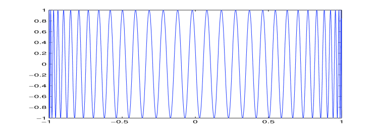
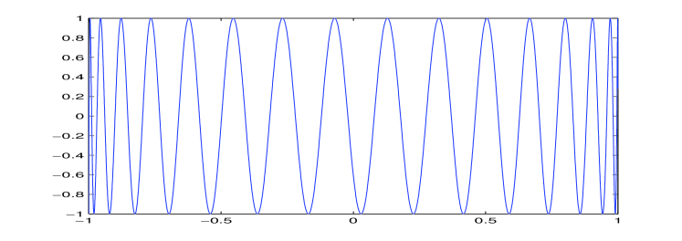
Our proposed multivariate algorithm combines a specific reducing transformation with the specialized univariate Hölder optimization algorithm MSPA developed in Section 2. The key idea is to define a parametric curve $C_{\alpha }:[0,T]\to D$, where $D\subset {ℝ}^n$ is the original search box, such that the curve $C_{\alpha }(t)=(c_1(t),\mathrm{\dots },c_n(t))$ is $\alpha$-dense in $D$. This property guarantees that for any point $x\in D$, there exists a $t\in [0,T]$ such that $\Vert C_{\alpha }(t)-x\Vert \le \alpha$.

Definition 4.

Let $𝕁$ be an interval of $ℝ$. We say that a parametrized curve of ${ℝ}^n$ defined by $C_{\alpha }:𝕁\to D=[a_1,b_1]\times \mathrm{\cdots }\times [a_n,b_n]$ is $\alpha$-dense in $D$, if for all $x\in D$, $\exists t\in 𝕁$ such that

$$d(x,C_{\alpha }(t))\le \alpha ,$$

where $d$ stands for Euclidean distance in ${ℝ}^n$.

By restricting the objective function $g$ to this curve, we obtain a univariate function $f:[0,T]\to ℝ$, defined by:

$$f(t)=g(C_{\alpha }(t)).$$

Crucially, if $g$ is Hölder continuous and $C_{\alpha }(t)$ is sufficiently regular (Lipschitz), the resulting function $f(t)$ is also Hölder continuous on the interval $[0,T]$. The original $n$-dimensional problem (1) is thus effectively reduced to the one-dimensional problem:

(P) $$\underset{t\in [0,T]}{\min }f(t).$$

This univariate problem can be efficiently solved using the algorithm from Section 2. The quality of the approximation to the original problem depends on the density parameter $\alpha$ of the curve.

Theorem 5.

Let $C_{\alpha }(t)=(c_1(t),\mathrm{\dots },c_n(t))$ be a function defined from $[0,T]$ into $D$. Let $\alpha >0$ and $\mu$ denote the Lebesgue measure, such that:

1. ${(c_i)}_{1\le i\le n}$ are continuous and surjective.

2. ${(c_i)}_{2\le i\le n}$ are periodic with respective periods ${(p_i)}_{2\le i\le n}$.

3. For any interval $I\subset [0,T]$ and for any $i\in \{2,\mathrm{\dots },n\}$, we have:

Then, for $t\in [0,T]$, the function $C_{\alpha }(t)$ is a parametrized $\sqrt{n-1}\alpha$-dense curve in $D$. (The proof can be found in [24]).

Corollary 6.

Let $C_{\alpha }(t)=(c_1(t),\mathrm{\dots },c_n(t)):[0,\frac{\pi }{{\alpha }_1}]\to D$ a function defined by:

$$c_i(t)=\frac{a_i-b_i}{2}\cos ({\alpha }_{i}t)+\frac{a_i+b_i}{2},i=1,2,\mathrm{\dots },n,$$

where ${\alpha }_1,\mathrm{\dots },{\alpha }_n$ are given strictly positive constants satisfying the relationships

$${\alpha }_i\ge \frac{\pi }{\alpha }(b_{i-1}-a_{i-1}){\alpha }_{i-1},\forall i=2,\mathrm{\dots },n.$$

Then the curve defined by the parametric curve $C_{\alpha }(t)$ is $\sqrt{n-1}\alpha$-dense in $D$ [24].

Remark 7.

According to Corollary 6, the parametrized curve $C_{\alpha }(t)$ is $\alpha$-dense in the box $D$. Moreover, the function $C_{\alpha }$ is Lipschitz on $[0,\frac{\pi }{{\alpha }_1}]$ with constant:

$$L_{\alpha }=\frac{1}{2}{\left(\underset{}{\overset{𝑛}{\sum _{i=1}}}{(b_i-a_i)}^2{\alpha }_i^2\right)}^{1/2}.$$

$\alpha =0.1$

$\alpha =0.3$

$\alpha =0.1$

Figure 2. The densification of the square ${[-1,1]}^2$ and the cube ${[-1,1]}^3$ by the support of $\alpha$-dense curves with different values of $\alpha$.

Theorem 8.

The function $f(t)=g(C_{\alpha }(t))$ for $t\in [0,\frac{\pi }{{\alpha }_1}]$ is a Hölder function with constant $H_f=h_g{L}_{\alpha }^{1/\beta }$ and exponent $\beta >1$.

Proof.

For $t_1$ and $t_2$ in $[0,\frac{\pi }{{\alpha }_1}]$, we have

$$\left|f(t_1)-f(t_2)\right|=\left|g(C_{\alpha }(t_1))-g(C_{\alpha }(t_2))\right|\le h_g{\Vert C_{\alpha }(t_1)-C_{\alpha }(t_2)\Vert }^{1/\beta }.$$

As the function of the parametric curve $C_{\alpha }$ is Lipschitz on $[0,\frac{\pi }{{\alpha }_1}]$ with the constants $L_{\alpha }$, we have

$$\Vert C_{\alpha }(t_1)-C_{\alpha }(t_2)\Vert \le L_{\alpha }\left|t_1-t_2\right|,$$

then

$$\left|f(t_1)-f(t_2)\right|\le h_g{\left(L_{\alpha }\left|t_1-t_2\right|\right)}^{1/\beta },$$

hence

$$\left|f(t_1)-f(t_2)\right|\le h_g{L}_{\alpha }^{1/\beta }{\left|t_1-t_2\right|}^{1/\beta }.$$

∎

3.2. The Mixed RT-MSPA Method

For determine the global minimum of $g$ on $D$ the mixed RT-MSPA method consists of two steps: the reducing transformation step and the application of the MSPA algorithm to the function $f(t)$ on $[0,\frac{\pi }{{\alpha }_1}]$.

Algorithm 2 RT-MSPA with known value of $h_g$

$D=[a_1,b_1]\times \mathrm{\cdots }\times [a_n,b_n]$ the search box.

The multivariate objective function with known Hölder parameters $h_g>0$

and $\beta >1$. $\epsilon >0$ small accuracy of the global minimization.

First part: $C_{\alpha }(t)$ the parametric $\alpha$-dense curve in $D$.

$f(t)$ the univariate $H_f$-Hölder function.

Second part: $f_{opt}$ the best global minimum of $f$.

First part:

Define $C_{\alpha }(t)$, $t\in [0,\pi /{\alpha }_1]⟶D$

$\alpha ={\left(\frac{\epsilon }{2H_f}\right)}^{\beta }$, ${\alpha }_1=1$.

for $i=2$ to $n$ do

  ${\alpha }_i=\frac{\pi }{\alpha }(b_{i-1}-a_{i-1}){\alpha }_{i-1}$

end for$\mathrm{𝐞𝐧𝐝}\mathrm{𝐟𝐨𝐫}$

for $i=1$ to $n$ do

  $c_i(t)=\frac{a_i-b_i}{2}\cos ({\alpha }_{i}t)+\frac{a_i+b_i}{2}$

end for$\mathrm{𝐞𝐧𝐝}\mathrm{𝐟𝐨𝐫}$

$C_{\alpha }(t)=(c_1(t),c_2(t),\mathrm{\dots },c_n(t))$ and $f(t)=g(C_{\alpha }(t))$.

Second part:

Initialization

$[0,\pi ]$ the search interval

$k\leftarrow 2,\rho \leftarrow 2,t_1\leftarrow 0,t_2\leftarrow \pi$

Step k: $t_1,t_2,\mathrm{\dots },t_k$ are ordered such that .

for $i=2$ to $k$ do

  $[t_{i-1},t_i]\subset [0,\pi ]$

  if $f(t_{i-1})\ne f(t_i)$ then

   ${\theta }_i$, ${\mu }_i,{\vartheta }_i$ and $z_i$ are defined respectively in (5), (6) and (7) (with respect to the variable $t>0$.)

  else

   $z_i=\frac{t_{i-1}+t_i}{2}$

  end if$\mathrm{𝐞𝐧𝐝}\mathrm{𝐢𝐟}$

  ${𝐌}_i=\min \{f(t_{i-1})-H_f{(z_i-t_{i-1})}^{1/\beta },f(t_i)-H_f{(t_i-z_i)}^{1/\beta }\}$

end for$\mathrm{𝐞𝐧𝐝}\mathrm{𝐟𝐨𝐫}$

${𝐌}_{\rho }=\min \left\{{𝐌}_i:2\le i\le k\right\}$

$t_{\rho }=z_{\rho }$

if $\left|t_{\rho }-t_{\rho -1}\right|>\epsilon$ then

  $t_{k+1}=z_{\rho }$

  $k⟵k+1$

  go to the Step $k$

else

  $f_{opt}=min\{f(t_i):1\le i\le k\}$

  Stop

end if$\mathrm{𝐞𝐧𝐝}\mathrm{𝐢𝐟}$

return $f_{opt}$

3.3. Convergence Result of RT-MPSA

Theorem 9.

Let $g$ be a Hölder function satisfying the condition (2) over $D$ and $𝐦$ be the global minimum of $g$ on $D$. Then the mixed RT-MSPA algorithm converges to the global minimum with an accuracy at least equal to $\epsilon$.

Proof.

Denote by ${𝐦}^{\ast }$ the global minimum of $f$ on $[0,\frac{\pi }{{\alpha }_1}]$, where $f(t)=g(C_{\alpha }(t)).$ On the other hand, let us designate by $f_{\epsilon }$ the global minimum of the problem $(P)$ obtained by the mixed method RT-MSPA. Let us show that

$$f_{\epsilon }-𝐦\le \epsilon .$$

1. As $g$ is continuous on $D$, there exists a point $𝐱\in D$ such that $𝐦=g(𝐱).$ Moreover, there exists $t_0\in [0,\frac{\pi }{{\alpha }_1}]$ such that $\Vert 𝐱-C_{\alpha }(t_0)\Vert \le {\left(\frac{\epsilon }{2h_g}\right)}^{\beta }$ so that

   $$\Vert g(𝐱)-g(C_{\alpha }(t_0))\Vert \le \frac{\epsilon }{2}.$$

   And therefore

   $$g(C_{\alpha }(t_0))-𝐦\le \frac{\epsilon }{2}.$$

   But from $𝐦\le {𝐦}^{\ast }\le g(C_{\alpha }(t_0))$, we deduce that

   (22) $${𝐦}^{\ast }-𝐦\le \frac{\epsilon }{2}.$$

2. As $f$ is continuous on $[0,\frac{\pi }{{\alpha }_1}],$ there exists a point $t^{\ast }\in [0,\frac{\pi }{{\alpha }_1}]$ such that ${𝐦}^{\ast }=f(t^{\ast })$, involving $t^{\ast }$ as a global minimizer of $f$. Then $t^{\ast }$ is a limit point of the sequence ${(t_k)}_{k\ge 1}$ obtained by the mixed algorithm.

   Hence $t^{\ast }\in [t_{\rho (k)-1},t_{\rho (k)}]$ and $\underset{k\to +\mathrm{\infty }}{lim}(t_{\rho (k)}-t_{\rho (k)-1})=0$. i.e.,

   On the other hand, since $f_{\epsilon }$ is the global minimum obtained after $k$ iterations, we obtain:

   $$\exists t_{\epsilon }\in [t_{s-1},t_s]:\left|t_s-t_{s-1}\right|\le {\left(\frac{\epsilon }{2H_f}\right)}^{\beta }\text{ and }{f}_{\epsilon }=f(t_{\epsilon })$$

   so that

   $$\{\begin{array}{c}{𝐌}_s=\min \{f(t_{s-1})-H_f{\left(t_{\epsilon }-t_{s-1}\right)}^{1/\beta },f(t_s)-H_f{\left(t_s-t_{\epsilon }\right)}^{1/\beta }\},\hfill \\ {𝐌}_s\le f(t^{\ast })\le f(t_{\epsilon })\text{and}{t}^{\ast }\in [t_{s-1},t_s].\hfill \end{array}$$

   Consequently,

   (23) $$f_{\epsilon }-{𝐦}^{\ast }=f(t_{\epsilon })-f(t^{\ast })\le H_f{\left|t_{\epsilon }-t^{\ast }\right|}^{1/\beta }\le \frac{\epsilon }{2}.$$

Finally, from (22) and (23), the result of Theorem 9 is proved. ∎

4. Numerical experiments

This section details the numerical experiments conducted to evaluate the performance of the proposed MSPA algorithm against existing methods, specifically SPA [12] and TPA [5], [8]. Two series of standard test functions and their corresponding data are listed in Table 1 and Table 4. Most of them have different properties like non-convex, non-differentiable and have more than at least two local and global minima. The evaluation covers both single-variable and multivariate optimization problems.

For all single-variable experiments, the desired accuracy for locating the global minimum was set to $\epsilon ={10}^{-4}(b-a)$, where $[a,b]$ is the search interval.

The primary performance criterion used for comparison are the total number of function evaluations ($Ev$) required and the CPU execution time in seconds ($T(s)$). Detailed results for the known and estimated Hölder constant are presented in Table 2 and Table 3, respectively. Within these tables, results shown in bold indicate the best performance achieved among the compared algorithms for each criterion ($Ev$ and $T(s)$) on a given test problem.

For multivariate optimization, we implemented the Reducing Transformation (RT) approach combined with the MSPA algorithm, utilizing $\alpha$-dense curves with a density parameter $\alpha =0.1$. Comparative results for The known and estimated Hölder constant are presented in Table 5 and Table 6, respectively.

The experiments were implemented in MATLAB and performed on a PC.

$N^{\circ }$	Function	Interval	Hölder constant $h_f$	Ref.
1	$\min \{\sqrt{\left|x+4\right|}-1,\sqrt{\left|x+1\right|}-1.005,\sqrt{\left|x-3\right|}+0.5\}$	$[-5,5]$	$2$	[21]
2	$\left|1.5-1.5\sqrt{\left|1-x^2\right|}\right|$	$[-2,2]$	$4$	$new$
$3$		$[0,6]$	$9.798$	[7]
4		$[0,1]$	$1.35$	$new$
5		$[0,1]$	$12.5$	$new$
6	$-\sqrt{1-x^2}$	$[-0.5,0.5]$	$\sqrt{2}$	[20]
7	$-\frac{2\sin x-1}{\sqrt{\left|x+1\right|}+2}$	$[-5,5]$	$7.8$	[5]
8	${\left|x-0.25\right|}^{\frac{2}{3}}-3\cos \frac{x}{2}$	$[-0.5,0.5]$	$4.26$	[14]
9	$-\cos \left(x\right)e^{\left(1-\frac{\sqrt{\left|\sin \left(\pi x\right)-0.5\right|}}{\pi }\right)}$	$[0,1]$	$4.3$	[14]
10	$5\cos x+\sqrt{0.8\left|x\right|}$	$[-10,8]$	$5.8$	$new$
11	$-\sqrt{\frac{9.5}{4}-x^2}-\frac{\sqrt{5}}{2}$	$[-1.5,1.5]$	$\sqrt{3}$	[14]
12	$-\cos \left(x+\frac{\pi }{2}-1\right)\exp \left(1-\frac{1}{\pi }\sqrt{\left|\sin \pi \left(x\frac{\pi }{2}-1\right)-0.5\right|}\right)$	$[-1.5,1.5]$	$7.3$	[14]
13	$-\left|\cos \left(\frac{\pi }{2}x\right)\right|{\left|\frac{\sqrt{19}-x}{\sqrt{2}-1}\right|}^{\frac{1}{2}}$	$[-1.5,1.5]$	$5.4$	[14]
14	$-\sqrt{1-{\sin }^{2}x}$	$[-1,1]$	$1$	$new$
15	$-\sqrt{16-{\cos }^{2}x}$	$[-2\pi ,2\pi ]$	$1$	$new$
16	$-\sqrt{1-x^2}+\sin x$	$[-1,1]$	$2.41$	$new$
17	$-{\left|8-x^3\right|}^{\frac{2}{3}}-\cos x-\sin 3x$	$[-2,2]$	$7.73$	$new$
18	$\sum _{k=1}^3\frac{1}{k}\left|\sin \left(\left(\frac{3}{k}+1\right)x+\frac{1}{k}\right)\right|{\left|x-k\right|}^{\frac{1}{2}}$	$[0,3]$	$6.83$	[15]
19	$-\sqrt{25-x^2}-shx$	$[-2.5,2.5]$	$8.36$	$new$
20	$-\frac{2\cos x-1}{\sqrt{\left|x+1\right|}+2}$	$[-5,5]$	$7.8$	$new$

Table 1. Univariate Hölder test functions.

Problem number		SPA		TPA		MSPA
$N^{\circ }$	$\beta$	$Ev$	$T\left(s\right)$	$Ev$	$T\left(s\right)$	$Ev$	$T\left(s\right)$
1	2	78	0.1167	74	0.0639	78	0.0655
2	2	2005	1.5050	2107	1.5976	2129	1.6245
3	2	4371	9.0077	2812	4.3383	3965	7.8945
4	2	254	0.1302	96	0.0711	104	0.0735
5	2	295	0.1940	79	0.0689	110	0.0957
6	2	3433	4.0167	3061	3.1928	3013	3.1567
7	2	4403	6.6673	4185	5.9728	4487	6.9423
8	3/2	87	0.0642	86	0.0636	89	0.0677
9	2	87	0.0657	86	0.0676	82	0.0650
10	2	704	0.2988	46	0.0653	696	0.2894
11	2	2867	2.8312	1721	1.1843	2149	1.6457
12	2	207	0.1419	216	0.0942	206	0.0905
13	2	1179	0.6164	1333	0.6984	1226	0.6143
14	2	2109	1.7937	1701	1.0748	1527	0.8923
15	2	3169	3.5469	3233	3.7415	3201	3.6079
16	2	2109	1.9788	1587	0.9685	1456	0.8341
17	3/2	668	0.6360	70	0.0637	697	0.2672
18	2	1342	0.7609	874	0.3612	864	0.3611
19	2	91	0.1198	83	0.0703	79	0.0688
20	2	2787	2.7692	1835	1.2205	1809	1.2010

Table 2. Comparison of results between MSPA and the existing algorithms with known value of $h_f$.

Problem number		SPAes		TPAes		MSPAes
$N^{\circ }$	$\beta$	$Ev$	$T\left(s\right)$	$Ev$	$T\left(s\right)$	$Ev$	$T\left(s\right)$
1	2	37	0.0116	48	0.0104	37	0.0064
2	2	1215	5.4778	962	3.5355	667	1.8018
3	2	2271	20.869	1819	13.717	1877	15.585
4	2	1288	6.4384	546	1.1884	240	0.2420
5	2	2854	31.324	575	1.2967	1104	4.8313
6	2	1501	8.6159	1841	12.972	1438	8.3665
7	2	1018	3.8064	1224	5.7721	1467	8.4715
8	3/2	22	0.0025	23	0.0026	21	0.0030
9	2	32	0.0049	31	0.0047	30	0.0044
10	2	986	3.7106	1062	4.3083	815	2.7356
11	2	1937	14.211	2446	22.842	2676	28.106
12	2	54	0.0126	69	0.0200	66	0.0194
13	2	1193	5.4486	914	3.2404	1364	7.3024
14	2	1391	7.3437	1707	11.168	1282	6.4865
15	2	1350	6.930	1540	9.0673	1045	4.3092
16	2	1995	15.269	1545	9.1268	1595	10.213
17	3/2	910	3.5283	638	1.7160	655	2.6685
18	2	578	1.2773	386	0.5728	437	0.7776
19	2	77	0.0246	74	0.0231	66	0.0191
20	2	687	1.7730	748	2.1631	553	1.2303

Table 3. Comparison of results between MSPA_es and the existing algorithms with unknown value of $h_f$.

$N^{\circ }$	Function	Box	Hölder constant $h_g$	Ref.
1	$\sum _{k=1}^3\frac{1}{k}\left|\cos \left(\left(\frac{3}{k}+1\right)\left(x+5\right)+\frac{1}{k}\right)\right|{\left|x-y\right|}^{\frac{1}{3}}$	${[-5,5]}^2$	$14.77$	[20]
2	$-\left|\cos \left(x\right)\cos \left(y\right)e^{\left(1-\frac{\sqrt{x^2+y^2}}{\pi }\right)}\right|$	$[-1,1]\times [-1,2]$	$5.0679$	[16]
3	$\sum _{k=1}^3\frac{1}{2k}\left|\cos \left(\left(\frac{3}{2k}+1\right)x+\frac{1}{2k}\right)\right|{\left|x-y\right|}^{\frac{2}{3}}$	${[-0.5,0.5]}^2$	$15.8$	[15]
4	${\left|x+y-0.25\right|}^{\frac{2}{3}}-3\cos \frac{x}{2}$	${[-0.5,0.5]}^2$	$4.26$	[15]
5	$-\cos \left(x\right)\sin \left(y\right)e^{\left(1-\frac{\sqrt{x^2+y^2}}{\pi }\right)}$	$[-1,1]\times [-1,2]$	$5.0679$	$new$
6	$max\{\sqrt{\left|x\right|},\sqrt{\left|y\right|}\}$	${[-1,1]}^2$	1	[3]
7	$\sqrt{\left|x\right|+\left|y\right|}$	${[-1,1]}^2$	${\left(\sqrt{2}\right)}^{\frac{1}{2}}$	[3]
8	$\sqrt{\left|x\right|}+\sqrt{\left|y\right|}$	${[-1,1]}^2$	$2$	[3]
9	$\sqrt{\left|x+1\right|}+\sqrt{\left|y+2\right|}+\sqrt{\left|z+\sqrt{6}\right|}$	${[-1,1]}^3$	$3$	$new$
10	$-10e^{-\sqrt{0.5\left(\left|x\right|+\left|y\right|\right)}}$	${[-2,12]}^2$	$\frac{10}{\sqrt{2}}$	[3]
11	$\left|3+\cos \left(\sqrt{x^2+y^2}\right)\right|$	${[-1,1]}^2$	$\sqrt{2}$	[16]
12	$\left|\sin \left(\sqrt{x^2+y^2}\right)\right|$	${[-1,1]}^2$	$\sqrt{2}$	[16]
13	$\frac{1}{2}\sin \left(\sqrt{\left|x-y\right|}\right)-\frac{1}{2}\sin \left(\sqrt{\left|x+y\right|}\right)$	$[0,1]\times [0,2.71]$	$1$	[16]
14	$\left|\cos \left(0.5+9.5\sqrt{x^2+y^2}\right)\right|$	${[-1,1]}^2$	$13.43$	[16]
15	$min\{\sqrt{\left|x+0.35\right|},\sqrt{\left|y+0.25\right|}\}$	${[-1,1]}^2$	$1$	$new$

Table 4. Multivariate Hölder test functions.

Problem number		RT-SPA		RT-TPA		RT-MSPA
$N^{\circ }$	$\beta$	$Ev$	$T\left(s\right)$	$Ev$	$T\left(s\right)$	$Ev$	$T\left(s\right)$
1	3	9131	28.642	8875	26.875	9055	28.103
2	2	1493	0.8627	1459	0.8278	1425	0.8030
3	3/2	6298	13.532	6255	13.316	6248	13.412
4	3/2	1053	0.4863	990	0.4411	986	0.4489
5	2	2844	2.8212	2770	2.6870	2692	2.600
6	2	218	0.0806	238	0.0868	213	0.0802
7	2	214	0.0769	196	0.0920	186	0.0734
8	2	331	0.1102	297	0.0997	319	0.1088
9	2	5795	11.432	5536	10.468	5507	10.501
10	2	4024	5.3531	4266	6.0112	3724	4.6304
11	2	2046	1.5416	2010	1.4863	1973	1.4524
12	2	509	0.1726	478	0.1615	475	0.1625
13	2	6309	13.646	6342	13.534	6257	13.335
14	2	6972	17.1265	6805	15.8143	6776	15.6564
15	2	497	0.1703	485	0.1682	480	0.1662

Table 5. Comparison of results between RT-MSPA and the existing algorithms with known value of $h_g$.

Figure 3. Illustration of the global minimization process and iteration points generated by RT-MSPA for function 12 (as defined in Table 4) on the domain ${[-1,1]}^2$.

Problem number			RT-SPAes		RT-TPAes		RT-MSPAes
$N^{\circ }$	$\beta$	$\lambda$	$Ev$	$T\left(s\right)$	$Ev$	$T\left(s\right)$	$Ev$	$T\left(s\right)$
1	3	2.1	2938	36.910	2460	26.040	2317	33.541
		1.07	1194	6.0336	/	/	1147	8.2836
2	2	1.5	665	1.6772	614	1.4797	607	1.4337
		1.07	435	0.7450	/	/	231	0.2266
3	3/2	1.5	636	1.7097	742	2.2662	732	3.2807
		1.07	466	0.926	/	/	286	0.5239
4	3/2	1.5	276	0.3303	267	0.3049	296	0.5407
		1.07	163	0.1200	/	/	136	0.1193
5	2	1.5	1595	9.6273	1765	11.474	1711	11.357
		1.07	1356	6.9890	/	/	1289	6.7921
6	2	3.1	610	1.4298	674	1.6995	591	1.3795
7	2	3.5	/	/	534	1.0745	506	1.0562
8	2	3.1	521	1.0367	1140	4.7631	529	1.1228
9	2	4.05	130	0.0697	/	/	33	0.0059
10	2	1.5	1723	11.188	2355	20.513	1966	15.084
		1.07	1530	8.9580	/	/	965	3.8254
11	2	14.4	290	0.3300	310	0.3749	310	0.3992
12	2	3.1	472	0.8553	459	0.7910	472	0.8762
13	2	1.5	134	0.0739	147	0.0855	145	0.0873
		1.07	79	0.02688	/	/	55	0.01473
14	2	1.5	2792	29.536	3134	36.0570	2923	32.761
15	2	1.5	84	0.0306	33	0.0055	53	0.0135

Table 6. Comparison of results between RT-MSPA_es and the existing algorithms with unknown value of $h_g$.

4.1. Discussions and remarks

The primary contributions of this paper are the development of MSPA, an enhanced version of Piyavskii’s algorithm for finding global minima of univariate Hölder continuous functions, and its extension, RT-MSPA, for solving higher-dimensional problems.

For the univariate problem, the comparison involves two cases based on the availability of the Hölder constant $h_f$:

• Known Hölder Constant ($h_f$): The standard SPA, TPA, and MSPA algorithms were used directly. The results are presented in Table 2.

• Unknown Hölder Constant ($h_f$): Modified versions of the algorithms, employing an estimation procedure for the Hölder constant, were used. These are denoted as SPA_es, TPA_es and MSPA_es, respectively. These versions utilize an estimate ${\tilde{h}}_f$ of the true Hölder constant $h_f$. The first remark in Table 3 that the results are obtained with the same value of $\lambda =1.5$ (multiplicative parameter) and $\nu ={10}^{-8}$ (tolerance parameter).

In higher-dimensional problems, comparative results are also presented for two cases, based on the availability of the Hölder constant $h_g$:

• Known Hölder Constant ($h_g$): The corresponding results are shown in Table 5 for the test problems listed in Table 4.

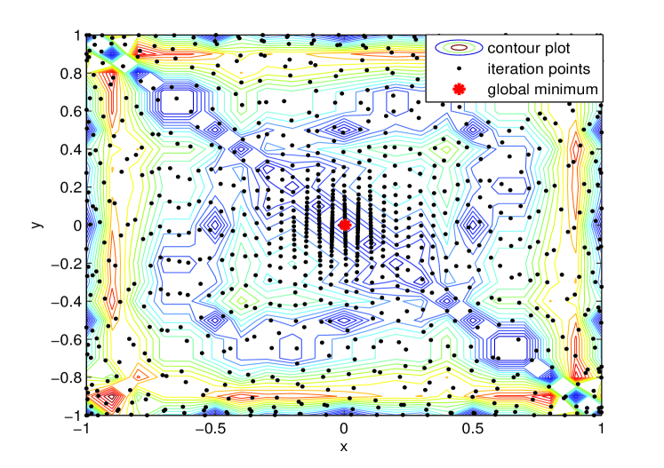
  In this context, Fig. 3 provides a numerical example illustrating how the RT-MSPA algorithm converges, by showing the iteration points produced by this algorithm around the global minimum.

• Unknown Hölder Constant ($h_g$): Table 6 presents a comparison between RT-MSPA_es and the corresponding estimation-based versions of existing algorithms (RT-SPA_es and RT-TPA_es), where $h_g$ is estimated.

  Moreover, in this case with the estimation of $h_g$, we observed that using $\nu ={10}^{-8}$ and $\lambda =1.07$ often yielded better results than $\lambda =1.5$. Notably, the RT-TPA_es method failed to produce results when $\lambda =1.07$.

It should be noted that for the multivariate tests in Table 6 (unknown $h_g$), two different values for the parameter $\lambda$ (typically $1.5$ and $1.07$) were generally used in the estimation procedure to obtain the reported results. The symbol (/) in Table 6 indicates instances where results could not be obtained for $\lambda =1.07$, particularly for the RT-TPA_es method.

Indeed, the TPA method (known $h_f$) is often faster and requires fewer evaluations according to Table 2, when comparing with SPA and MSPA. However, even in this case, the performance of MSPA remains competitive when compared to TPA. A possible reason for this is that for certain functions with a known Hölder constant $h_f$, the more aggressive linear approximation used by TPA is more effective at quickly locating the global minimum than the secant-based approximation of MSPA. This can be particularly true for functions where the Hölder exponent $\beta$ is close to 1, making the function’s behavior more linear.

In the case where $h_f$ is unknown a priori, the situation is different (see Table 3). Also, according to Table 5 and Table 6, in the cases where $h_g$ is known and $h_g$ is unknown, the performance of MSPA_es and RT-MSPA_es is more competitive compared to the other algorithms.

Finally, for problems with a known Hölder constant $h_f$, MSPA required 68.42% fewer function evaluations than SPA, and 50% fewer than TPA. It also achieved an 80% reduction in execution time compared to SPA, and 50% compared to TPA. When the Hölder constant is unknown, MSPA_es maintained strong performance, requiring 78.95% fewer evaluations than SPA_es, and 60% fewer than TPA_es, while also reducing execution time by 75% and 55%, respectively. Similarly, RT-MSPA_es demonstrated its efficiency for problems with an unknown constant $h_g$, achieving up to 61.9% fewer function evaluations than RT-SPA_es, and 85.71% fewer than RT-TPA_es, along with execution time reductions of 54.55% and 68.18%, respectively.

Based on these comparative studies, the MSPA, MSPA_es, RT-MSPA, and RT-MSPA_es algorithms demonstrate higher efficiency compared to the other techniques evaluated.

5. Conclusion

This paper addressed the global optimization of multivariate Hölderian functions defined on a box domain in ${ℝ}^n$. A key focus was the challenging yet practical case where the Hölder constant $h_g$ is unknown a priori. To tackle this class of problems, we developed and analyzed two novel algorithms: the MSPA and RT-MSPA. We provided rigorous mathematical proofs establishing the convergence guarantees for both proposed methods. To evaluate their practical efficacy, MSPA and RT-MSPA were implemented and tested on a suite of standard functions commonly used in global optimization literature. The numerical results were compared against those obtained by other well-known search methods. This comparative analysis demonstrated the viability and effectiveness of our approach, in particular, offers a competitive performance in practice. Future work could explore further adaptive strategies within the partitioning framework or extend the approach to handle different types of constraints.

Acknowledgements.

The authors would like to thank the anonymous referee for his useful comments and suggestions, which helped to improve the presentation of this paper.