Power series for the half width
of the Voigt function, rederived

Abstract.

The Voigt function is the convolution of a Gaussian and a Lorentzian. We rederive power series for its half width at half maximum for the limiting cases of near-Gaussian and near-Lorentzian line shapes. We thereby provide independent verification and slight corrections of the expansion coefficients reported by Wang et al (2022). Results are used in our implementation of function voigt_hwhm in the open-source library libcerf.

1. Introduction

The Voigt [8] function is the convolution of a Gaussian and a Lorentzian [5, 7.19.1]. It is frequently used to describe peak shapes in spectroscopy and diffraction. In such applications, it is customary to characterize peaks by their full or half width at half maximum (fwhm, hwhm).

Much work has been devoted to numerical approximations of the Voigt function and its half width. For most applications, considering experimental uncertainties, quite simple approximations would do. Nonetheless, for internal consistency and reproducibility of data analyses, to facilitate numerical differentiation (e.g., in fitting routines), and out of pure mathematical interest, it is worthwhile to push approximations to ever better accuracy.

The Voigt function can be expressed through the Faddeeva function, which is closely related to the complex error function. Therefore, our open-source complex error function library libcerf [4] also provides functions voigt and voigt_hwhm. Earlier versions of libcerf computed voigt_hwhm very directly by bisection on function values of voigt. Starting with release 3.3, a completely new implementation of voigt_hwhm uses series expansions for the near-Gaussian and near-Lorentzian limiting cases, and piecewise Chebyshev interpolation [10] in between. Near machine accuracy is achieved in each region. This paper documents the two series expansions.

The same series have recently been studied by Wang et al [9]. Here, we rederive them in different ways and thereby provide independent verification and slight corrections for the coefficients tabulated in [9]. For the near-Gaussian case, our derivation (Section 3) is more compact, as we use complex notation and represent the Voigt function through the Faddeeva function instead of decomposing it as in [9, Eq 9]. For the near-Lorentzian case, Wang et al chose a pragmatic method: numerical differentiation, followed by rounding to integer numerators [9, Appendix B]. Here (Section 4), we derive a fully algebraic recursion.

2. Foundations

2.1. Voigt function

The Voigt function

(1) $$V(q;\sigma ,\gamma )≔{\int }_{-\mathrm{\infty }}^{\mathrm{\infty }}dpG(p;\sigma )L(q-p;\gamma )$$

is the convolution of a normalized Gaussian with standard deviation $\sigma$

(2) $$G(q;\sigma )≔\frac{1}{\sqrt{2\pi }\sigma }\exp \left(-\frac{q^2}{2{\sigma }^2}\right)$$

and a normalized Lorentzian with half width $\gamma$

(3) $$L(q;\gamma )≔\frac{\gamma }{\pi \left({\gamma }^2+q^2\right)}.$$

As $G$ and $L$ are even functions of $\sigma$ and $\gamma$, so is $V$. Therefore in the following we will only consider $\sigma ,\gamma \ge 0$. Otherwise said, we will simply write $\sigma$ and $\gamma$ instead of their absolute values.

2.2. Half width

Function $H(\sigma ,\gamma )$ is the half width at half maximum of the Voigt function. It is implicitly defined by

(4) $$V(H(\sigma ,\gamma );\sigma ,\gamma )=\frac{1}{2}V(0;\sigma ,\gamma ).$$

Or, introduce the reduced Voigt function

(5) $$v(q;\sigma ,\gamma )≔\frac{V(q;\sigma ,\gamma )}{V(0;\sigma ,\gamma )},$$

and its inverse function $v^{-1}$ with respect to the first argument, such that

(6) $$v(q;\sigma ,\gamma )=y\iff v^{-1}(y;\sigma ,\gamma )=q.$$

Then we have simply

(7) $$H(\sigma ,\gamma )=v^{-1}(\frac{1}{2};\sigma ,\gamma ).$$

2.3. Scaling

For real $\alpha \ne 0$, the Voigt function scales as

(8) $$V(\alpha q;\alpha \sigma ,\alpha \gamma )=\frac{1}{\alpha }V(q;\sigma ,\gamma ).$$

The reduced Voigt function scales accordingly as

(9) $$v(\alpha q;\alpha \sigma ,\alpha \gamma )=v(q;\sigma ,\gamma ),$$

and its inverse as

(10) $$v^{-1}(y;\alpha \sigma ,\alpha \gamma )=\alpha v^{-1}(y;\sigma ,\gamma ).$$

This implies for the half width

(11) $$H(\alpha \sigma ,\alpha \gamma )=\alpha H(\sigma ,\gamma ).$$

The homogeneity of degree 1 implies that we only need to study a function of one real variable $\sigma /\gamma$ or $\gamma /\sigma$.

2.4. Relation to the Faddeeva function

Given the error function

(12) $$\mathrm{erf}(z)≔\frac{2}{\sqrt{\pi }}{\int }_0^{z}dt{\mathrm{e}}^{-t^2},$$

the complementary error function

(13) $\mathrm{erfc}(z)$ $≔1-\mathrm{erf}(z)$

(14) $={\displaystyle \frac{2}{\sqrt{\pi }}}{\displaystyle {\int }_z^{\mathrm{\infty }}}dt{\mathrm{e}}^{-t^2},$

and the underflow-compensated complementary error function

(15) $$\mathrm{erfcx}(z)≔{\mathrm{e}}^{z^2}\mathrm{erfc}(z),$$

the Faddeeva function is [5, 7.2.3]

(16) $w(z)$ $=\mathrm{erfcx}(-iz)$

(17) $=e^{-z^2}\mathrm{erfc}(-iz)$

(18) $={\mathrm{e}}^{-z^2}{\displaystyle \frac{2}{\sqrt{\pi }}}{\displaystyle {\int }_{-iz}^{\mathrm{\infty }}}dt{\mathrm{e}}^{-t^2}$

(19) $={\mathrm{e}}^{-z^2}\left(1-{\displaystyle \frac{2}{\sqrt{\pi }}}{\displaystyle {\int }_0^{-iz}}dt{\mathrm{e}}^{-t^2}\right)$

(20) $={\mathrm{e}}^{-z^2}\left(1+i{\displaystyle \frac{2}{\sqrt{\pi }}}{\displaystyle {\int }_0^z}dt{\mathrm{e}}^{t^2}\right).$

Another integral representation, valid for $\mathrm{Im}z>0$, is [5, 7.7.2]

(21) $$w(z)=\frac{i}{\pi }{\int }_{-\mathrm{\infty }}^{+\mathrm{\infty }}dt\frac{{\mathrm{e}}^{-t^2}}{z-t}.$$

Let us define $u≔\mathrm{Re}w$ and $v≔\mathrm{Im}w$ so that

(22) $$w(z)\equiv u(z)+iv(z).$$

The real part of Eq. 21 is

(23) $$u(x+iy)=\frac{y}{\pi }{\int }_{-\mathrm{\infty }}^{+\mathrm{\infty }}dt\frac{{\mathrm{e}}^{-t^2}}{{(x-t)}^2+y^2},$$

which is essentially Voigt’s convolution integral Eq. 1. Divide $t$, $x$, and $y$ by $\sqrt{2}\sigma$ to find

(24) $V(q;\sigma ,\gamma )={\displaystyle \frac{1}{\sqrt{2\pi }\sigma }}u\left({\displaystyle \frac{q}{\sqrt{2}\sigma }}+i{\displaystyle \frac{\gamma }{\sqrt{2}\sigma }}\right).$

Accordingly, the Voigt half width is implicitly defined by a functional equation that involves the real part of Faddeeva’s function,

(25) $u\left({\displaystyle \frac{H(\sigma ,\gamma )}{\sqrt{2}\sigma }}+i{\displaystyle \frac{\gamma }{\sqrt{2}\sigma }}\right)={\displaystyle \frac{1}{2}}u\left(i{\displaystyle \frac{\gamma }{\sqrt{2}\sigma }}\right).$

3. Near-Gaussian case $𝜸\mathbf{\ll }𝝈$

3.1. Case $𝜸\mathbf{=}\mathrm{𝟎}$

In the case $\gamma =0$, the Voigt function is just a Gaussian with standard deviation $\sigma$. With a real argument $z=x$, the real part of Eq. 20 is simply

(26) $$u(x)={\mathrm{e}}^{-x^2}.$$

The implicit equation Eq. 25 is solved by the well-known

(27) $$H(\sigma ,0)=\sqrt{2\ln 2}\sigma .$$

3.2. Rescaled function $𝒇$

We now consider the case of a relatively small Lorentzian width, $\gamma \ll \sigma$. Thanks to the scaling property Eq. 11, the half width of the Voigt function can be computed as

(28) $$H(\sigma ,\gamma )=\sigma H(1,\gamma /\sigma ).$$

For later convenience, we introduce the reduced variable

(29) $$t≔\frac{\gamma }{\sqrt{2}\sigma }$$

so that

(30) $$H(\sigma ,\gamma )=\sigma H(1,\sqrt{2}t).$$

We define the function

(31) $$f(t)≔\frac{H(1,\sqrt{2}t)-H(1,0)}{\sqrt{2}}+it$$

and the constant

(32) $$\eta ≔\frac{H(1,0)}{\sqrt{2}}=\sqrt{\ln 2}$$

so that $H(\sigma ,\gamma )$ can be obtained via Eq. 30 and

(33) $$H(1,\sqrt{2}t)=\sqrt{2}\left(\eta +f(t)-it\right).$$

Below, we will determine a series expansion for $f(t)$, so that we can ultimately compute the Voigt width using

(34) $$H(1,\sqrt{2}t)=\sqrt{2}\left(\eta +\sum _{n=1}^{\mathrm{\infty }}(\mathrm{Re}{f}_n)t^n\right).$$

3.3. Power series in $𝒕$ and $𝒇$

In Eq. 25, choose $\sigma =1$ and $\gamma =\sqrt{2}t$. then use Eq. 30 and Eq. 33 to obtain an implicit equation for $f$,

(35) $$u\left(\eta +f(t)\right)=\frac{1}{2}u\left(it\right).$$

On the right-hand side, use the Maclaurin expansion of $w(z)$ [5, 7.6.3] to obtain

(36) $$u(it)=\sum _{n=0}^{\mathrm{\infty }}\frac{{(-t)}^n}{\mathrm{\Gamma }\left(\frac{n}{2}+1\right)}.$$

On the left-hand side of Eq. 35, use the Taylor expansion

(37) $$u\left(\eta +f(t)\right)=\mathrm{Re}\sum _{n=0}^{\mathrm{\infty }}{w}_{n}f{(t)}^n$$

with coefficients

(38) $$w_n≔\frac{w^{(n)}(\eta )}{n!}$$

given by the recursion [5, 7.10.3] [7, Eq 10]

(39) $$w_n=-\frac{2}{n}\left(\eta w_{n-1}+w_{n-2}\right)$$

with starting values $w_0≔w(\eta )$ and $w_{-1}≔-i/\sqrt{\pi }$.

Combine Eqs. 35, 36 and 37, and omit terms in $t^0$, to obtain an equation that relates the power series in $t$ and in $f$,

(40) $$\frac{1}{2}\sum _{n=1}^{\mathrm{\infty }}\frac{{(-t)}^n}{\mathrm{\Gamma }\left(\frac{n}{2}+1\right)}=\sum _{n=1}^{\mathrm{\infty }}\mathrm{Re}{w}_{n}f{(t)}^n.$$

3.4. Recursive solution

To solve Eq. 40 numerically, function $f(t)$ shall be expressed as a power series in $t$. Since $f(0)=0$ by construction Eq. 31, the power series starts with the linear term,

(41) $$f(t)\equiv \sum _{n=1}^{\mathrm{\infty }}{f}_n{t}^n.$$

Per Eq. 31, the $f_n$ are real for $n>1$; only for $n=1$ there is an imaginary part, per the definition Eq. 31, so that

(42) $$\mathrm{Im}{f}_n={\delta }_{n1}.$$

With notation from [3], write $[t^N]f(t)$ for the coefficient of $t^N$ in the power series representing $f(t)$. For the series Eq. 41, $[t^N]f(t)=f_N$. Define

(43) $$F_{N,n}≔\left[t^N\right]f{(t)}^n,$$

and apply the operator $[t^N]$ to both sides of Eq. 40:

(44) $$\frac{{(-1)}^N}{2\mathrm{\Gamma }(\frac{N}{2}+1)}=\sum _{n=1}^N\mathrm{Re}{w}_n{F}_{N,n}$$

for all $N\ge 1$.

Equations Eqs. 44, 43 and 41 fully determine the $f_n$ in terms of the $w_n$, which are given by the recursion Eq. 39. We resolve said equations in two steps. First, we solve Eq. 44 for $F_{N,1}$. For $N=1$, we recall Eq. 42 to obtain

(45) $$F_{1,1}={(\mathrm{Re}{w}_1)}^{-1}\left(\mathrm{Im}{w}_1-\frac{1}{2\mathrm{\Gamma }(\frac{3}{2})}\right)+i.$$

For $N>1$,

(46) $$F_{N,1}={(\mathrm{Re}{w}_1)}^{-1}\left(\frac{{(-1)}^N}{2\mathrm{\Gamma }(\frac{N}{2}+1)}-\sum _{n=2}^N\mathrm{Re}{w}_n{F}_{N,n}\right).$$

Second, we use Eq. 41 to obtain the $F_{N,n}$ for $n>1$:

(47) $$F_{N,n}=\sum _{m=1}^{N-n+1}{F}_{m,1}{F}_{N-m,n-1}.$$

Finally, we note that the coefficients of Eq. 41 are $f_N\equiv F_{N,1}$. This completes our derivation of a power series for the half width $H$.

To minimize the number of computational operations in the highly optimized code of libcerf, we write Eqs. 28 and 34 as

(48) $$H(\sigma ,\gamma )=\sigma \sqrt{2\ln 2}+\gamma \sum _{n=0}^{N_{\text{cut}}}{c}_n{\left(\frac{\gamma }{\sigma }\right)}^n$$

with precomputed coefficients

(49) $$c_n≔\frac{\mathrm{Re}{f}_{n+1}}{{\sqrt{2}}^n}.$$

3.5. Implementation

A Python script near_gauss.py used to generate coefficients is preserved in subdirectory dev/voigt of the libcerf source repository. The script uses the arbitrary-precision math library mpmath [6] with a fixed internal precision, checked against a computation with some more digits. It turns out that an internal precision of 40 decimal digits is needed to compute $f_n$ for with 32 reliable decimal digits. The program executes within a fraction of a second.

The recursive forward computation of $w_n$ according to Eq. 39 would be divergent if $\eta$ had a positive imaginary part [7]. In our case, $\eta$ is real so that we are at the margin of numerical instability. Indeed, our computations show that up to $n=30$ only the last few decimal digits get incorrect. Nonetheless, our script validates each $w_n$ against a non-recursive computation, derived in the Appendix.

3.6. Results

Table 1. Coefficients $f_n$ of the series Eq. 41 that can be used according to Eq. 33 for computing the half width $H(\sigma ,\gamma )$ in the near-Gaussian case of $\gamma \ll \sigma$. Digits that deviate from [9, Table A1] are underlined. Agreement through $n=22$ confirms essential correctness of both their work and ours.

Resulting coefficients $f_n$ up to $n=30$ are reported in Table 1 with 32 digits precision. Up to $n=22$, they fully agree with [9, Table A1]. Then, suddenly, the agreement drops to 12 digits for $f_{23}$, and further decreases to 7 digits for $f_{30}$. Given that our algorithm is simpler than the one of [9] and that we cross-checked our results with different internal accuracies we are confident that all digits reported in Table 1 are correct.

4. Near-Lorentzian case $𝝈\mathbf{\ll }𝜸$

4.1. Case $𝝈\mathbf{=}\mathrm{𝟎}$

For a pure Lorentzian, $V(q;0,\gamma )=L(q;\gamma )$, the half width is just $H(0,\gamma )=\gamma$.

4.2. Rescaled function $𝒈$

We now consider the case of a relatively small Gaussian width, $\sigma \ll \gamma$. Thanks to the scaling property Eq. 11, the half width of the Voigt function can be computed as

(50) $$H(\sigma ,\gamma )=\gamma H(\sigma /\gamma ,1).$$

For later convenience, we introduce a reduced variable

(51) $$s≔{\sigma }^2/{\gamma }^2$$

and a real function

(52) $$g(s)≔H(\sqrt{s},1)-1=H(\sigma /\gamma ,1)-1=\frac{H(\sigma ,\gamma )-\gamma }{\gamma }$$

that is to be determined so that we ultimately obtain the Voigt half width as

(53) $$H(\sigma ,\gamma )=\gamma \left(1+g\left({\sigma }^2/{\gamma }^2\right)\right).$$

In this notation, the implicit definition Eq. 25 of $H$ can be written as

(54) $$2u\left(\frac{1+g(s)+i}{\sqrt{2s}}\right)-u\left(\frac{i}{\sqrt{2s}}\right)=0,$$

which needs to be resolved for $g$.

For large $|z|$, the Faddeeva function can be computed from its asymptotic expansion [1, p. 14]

(55) $$w(z)=\frac{i}{\sqrt{\pi }}\sum _{n=0}^N\frac{a_n}{2^n{z}^{2n+1}}+R_N(z)$$

with the abbreviation

(56) $$a_n≔\frac{2^n}{\sqrt{\pi }}\mathrm{\Gamma }\left(n+1/2\right)=\frac{(2n)!}{2^{n}n!}=(2n-1)!!.$$

The remainder $|R_N|$ is no larger than the first term omitted from the sum. Drop the explicit notation of truncation, and apply Eq. 55 to Eq. 54,

(57) $$0\simeq \mathrm{Im}\sum _{n=0}^{\mathrm{\infty }}\frac{a_n}{2^n}\left\{2{\left(\frac{\sqrt{2s}}{1+g+i}\right)}^{2n+1}-{\left(\frac{\sqrt{2s}}{i}\right)}^{2n+1}\right\}.$$

Factor out ${(2s)}^n$, and drop a common factor $\sqrt{2s}$:

(58) $$0\simeq \mathrm{Im}\sum _{n=0}^{\mathrm{\infty }}{a}_n\left\{2{\left(\frac{1}{1+g+i}\right)}^{2n+1}-{\left(\frac{1}{i}\right)}^{2n+1}\right\}{s}^n.$$

Binomial expansion:

(59) $$0\simeq \mathrm{Im}\sum _{n=0}^{\mathrm{\infty }}{a}_n\left\{2{\left(\frac{1}{1+i}\right)}^{2n+1}\sum _{k=0}^{\mathrm{\infty }}\left(\genfrac{}{}{0pt}{}{2n+k}{k}\right){\left(\frac{-g}{1+i}\right)}^k-{\left(\frac{1}{i}\right)}^{2n+1}\right\}{s}^n.$$

As $a_n$, $s$, $g$ are all real, the only complex quantity here is the imaginary unit $i$.

We precompute

(60) $${(-1)}^k\mathrm{Im}{\left(\frac{1}{1+i}\right)}^{2n+k+1}=\frac{{\psi }_{2n+k}}{4\cdot 4^{\lfloor (2n+k)/4\rfloor }},$$

where ${\psi }_k$ is an integer function with period 8, given by

(61) $$({\psi }_0,{\psi }_1,\mathrm{\dots },{\psi }_7)≔(2,-2,1,0,-2,2,-1,0).$$

Multiply Eq. 59 by 2 and use Eq. 60 to obtain

(62) $$0\simeq \sum _{n=0}^{\mathrm{\infty }}{a}_n\left\{\sum _{k=0}^{\mathrm{\infty }}{b}_{n,k}{g}^k-2{(-1)}^n\right\}{s}^n.$$

with the rational function

(63) $$b_{n,k}≔\left(\genfrac{}{}{0pt}{}{2n+k}{k}\right)\frac{{\psi }_{2n+k}}{4^{\lfloor (2n+k)/4\rfloor }}.$$

4.3. Solution

We seek a solution in form of a power series

(64) $$g(s)=\sum _{j=1}^{\mathrm{\infty }}{g}_j{s}^j.$$

As in Section 3.4, write $[s^n]f$ for the coefficient of $s^n$ in a power series representing $f(s)$. Apply the operator $[s^n]$ to Eq. 62:

(65) $$0\simeq \sum _{m=0}^{\mathrm{\infty }}{a}_m\left\{\left(b_{m,0}-2{(-1)}^m\right)+[s^{n-m}]\sum _{k=1}^{\mathrm{\infty }}{b}_{m,k}{g}^k\right\}.$$

Define

(66) $$G_{N,m}≔\left[s^N\right]g^m.$$

Restrict the sums to non-zero terms, using the fact that $g(s)$ per Eq. 64 has no $s^0$ term:

(67) $$0\simeq a_n\left(b_{n,0}-2{(-1)}^n\right)+\sum _{m=0}^n{a}_m\sum _{k=1}^{n-m}{b}_{m,k}{G}_{n-m,k}.$$

The only linear occurrence of $g_n\equiv G_{n,1}$ is in the $m=0,k=1$ term, with prefactor $a_0{b}_{0,1}=-2$. Isolating that contribution gives the recurrence

(68) $$G_{n,1}=\frac{1}{2}\left\{a_n\left(b_{n,0}-2{(-1)}^n\right)+\sum _{m=0}^n{a}_m\sum _{k=1+{\delta }_{m0}}^{n-m}{b}_{m,k}{G}_{n-m,k}\right\}.$$

The recurrence starts from

(69) $$G_{1,1}=\frac{a_1(b_{1,0}+2)}{2}=\frac{3}{2}.$$

Coefficients $G_{n,k}$ with can be computed by another recursion, as in Eq. 47 of Section 3.4,

(70) $$G_{n,k}=\sum _{j=1}^{n-k+1}{G}_{j,1}{G}_{n-j,k-1}.$$

While the coefficients $a,c$ in Eq. 68 are integers, the $b$ are rational numbers with denominators that are powers of 2. Therefore the $g_n\equiv G_{n,1}$ must also be rational numbers, and their denominators powers of 2.

4.4. Implementation

A Python script near_lorentz.py used to generate coefficients is preserved in subdirectory dev/voigt of the libcerf source repository. The script employs the Python library Fraction to compute exact rational numbers using long-integer arithmetics.

4.5. Results

Table 2. Coefficients $g_n$ of the asymptotic expansion Eq. 64 that can be used according to Eq. 53 for computing the half width $H(\sigma ,\gamma )$ in the near-Lorentzian case of $\sigma \ll \gamma$. Based on these $g_n$, we can confirm the $T_{2n}$ of [9, Table A2] except for $n=15$, as discussed in Section 4.5.

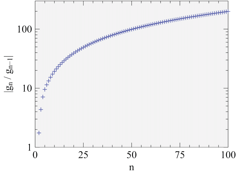
The expansion coefficients $g_n$ are reported in Table 2. The ratio of consecutive coefficients is shown as $\log |g_n/g_{n-1}|$ versus $n$ in Figure 1, which indicates that the $|g_n|$ grow faster than a power law. In consequence, Eq. 64 is an asymptotic series, as was noted by Wang et al [9], and was to be expected from the asymptotic expansion Eq. 55 used for $w(z)$.

Figure 1. Absolute value of the ratio of consecutive coefficients, $|g_n/g_{n-1}|$, shown on a logarithmic scale against $n$. The ratio appears to grow slowly beyond all limits.

Wang et al expanded squared half widths in a series [9, Eq A30] that reads in our notation

(71) $${\left(\frac{H(\sigma ,\gamma )}{\gamma }\right)}^2=\sum _{n=0}^{\mathrm{\infty }}{T}_n\left(\frac{\sigma }{\sqrt{2}\gamma }\right)=\sum _{n=0}^{\mathrm{\infty }}{T}_n\left(\sqrt{\frac{s}{2}}\right).$$

They computed rational numbers $T_n$ by approximating floating-point numbers obtained from numerical differentiation [9, Eq A31]. For odd $n$, they found $T_n=0$, consistent with our Eqs. 53 and 64. To validate their results for even $n$, we recompute $T_{2m}$ as

(72) $$T_{2m}=\left[{\left(\frac{s}{2}\right)}^m\right]{\left(\frac{H(\sigma ,\gamma )}{\gamma }\right)}^2=2^m\left[s^m\right]{\left(1+g(s)\right)}^2.$$

We define $g_0≔1$ so that we are left with a self-convolution

(73) $$T_{2m}=2^m\left[s^m\right]{\left(\sum _{k=0}^{\mathrm{\infty }}{g}_k{s}^k\right)}^2=2^m\sum _{k=0}^m{g}_k{g}_{m-k}.$$

With rational arithmetics based on our $g_k$ as shown in Table 2, we confirm the $T_{2m}$ of [9, Table A2] except for their $T_{30}=176955754371862947/2^{19}$, which is too large by $3/2^{20}$; the correct result is $353911508743725891/2^{20}$.

Appendix. Closed expression for ${𝒘}_{𝒏}$

As the recursion Eq. 39 is marginally unstable, it may be preferable to compute $w_n$ from a closed expression, or at least use the direct computation as a cross-check. With Eqs. 38 and 17,

(74) $$w_n=\frac{1}{n!}\frac{{\mathrm{d}}^n}{\mathrm{d}{(-iz)}^2}{\mathrm{e}}^{{(-iz)}^2}\mathrm{erfc}(iz).$$

With [5, 7.18.4], [2, 2.23], and with the notation ${\text{i}}^n\mathrm{erfc}$ [5, 7.18.2] for the iterated integral of erfc,

(75) $$w_n=i^n{2}^n{\mathrm{e}}^{{(-iz)}^2}{\text{i}}^n\mathrm{erfc}(-iz).$$

With [5, 7.18.11],

(76) $$w_n=i^n{2}^n\frac{{\sqrt{2}}^{n-1}}{\sqrt{\pi }}{\mathrm{e}}^{z^2/2}U(n+1/2,-i\sqrt{2}z).$$

The parabolic cylinder function $U$ [5, Chapter 12] is provided by mpmath as the function pcfu. Internally, mpmath computes it by means of hypergeometric functions.