APPROXIMATION AND NUMERICAL RESULTS FOR PHASE FIELD SYSTEM BY A FRACTIONAL STEP SCHEME
COSTICÃ MOROŞANU
(Iaşi)
(Iaşi)
1. INTRODUCTION
We consider the phase field system
subject to the Dirichlet boundary conditions and initial conditions
where
Setting
system (1.1)-(1.4) takes the form
Let
Define the operator
and the operator
Thus, system (1.6)-(1.7) can be rewritten in the form
For others settings into the abstract framework of the phase-field equations (1.1)-(1.4) see, e.g., [6], [14].
The idea behind the Lie-Trotter scheme (known as the method of fractional step in numerical approximation of PDE's) is to decompose the original problem into several simpler problems.
Here we associate to system (
where
Recall that
accretive, if for every pair
accretive, if for every pair
or, equivalently,
where
Another convenient way to define the accretiveness is obtained using
i.e, (ii) can be equivalently written as
(ii')
(ii')
(see also [2], [15], [16]). Recall that if
It is well known that, under certain hypotheses on
has a generalized solution
for every
This is the sense in which we will treat the problems (1.6)-(1.9) and (1.10)-(1.13).
This is the sense in which we will treat the problems (1.6)-(1.9) and (1.10)-(1.13).
2. CONVERGENCE OF THE APPROXIMATE SCHEME
Let us recall the following result due to Barbu and Iannelli ([5]).
THEOREM 2.1. Let
(H1)
(H2)
THEOREM 2.1. Let
(H1)
(H2)
(H3)
(H4) For every
(H4) For every
Then, for every
and the limit is uniform on bounded
Here, by
Here, by
and by
This result is not applicable to the problem (1.10)-(1.13) because we cannot find a subset
This result is not applicable to the problem (1.10)-(1.13) because we cannot find a subset
Therefore, we will replace the operator
Fig. 1
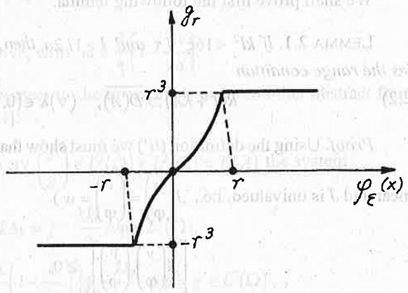
where
Substituting in
We associate to system (
Now we prove
Proposition 2.1. If
Proposition 2.1. If
We shall prove first the following lemma.
Lemma 2.1. If
Lemma 2.1. If
Proof. Using the definition (ii') we must show that, for every
Using Green formula and Cauchy-Schwarz's inequality, we get (
Since
Thus, because
i.e.
Hence
Other results with respect to the operator
Other results with respect to the operator
It is clear that for every
has a unique solution
The proof of Proposition 2.1. By Proposition 3.9 pp. 110 ([2]), we have that
Remark 2.1. If we can choose
and the solution of the approximate problem (
3. NUMERICAL RESULTS
We consider
Denote by
As well, we denote by
Using a standard implicit scheme, (1.6)-(1.7) are discretized as
and
where
Setting
Setting
(3.1) and (3.2) can be rewritten for the level of time
with
and
Let
Let
System (3.3) takes the form
where
Thus we have to solve the nonlinear system
Thus we have to solve the nonlinear system
Using the Newton iterative method to solve it, we have
where
Using an implicit scheme and the Newton iterative method, we obtain from (2.1)
where
Using the very same way of discretization and implicit scheme, the approximative version of (1.10) is given by
and
with
For fixed
For fixed
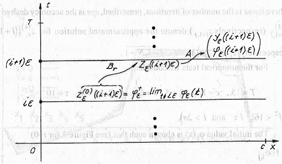
Fig. 2
and, the numerical algorithm to calculate it, can be obtained by the following sequence
next
sol:
sol:
Solve the linear system (3.7)
where itmax is the number of iterations, prescribed, eps is the accuracy desired and
For the numerical tests we consider:
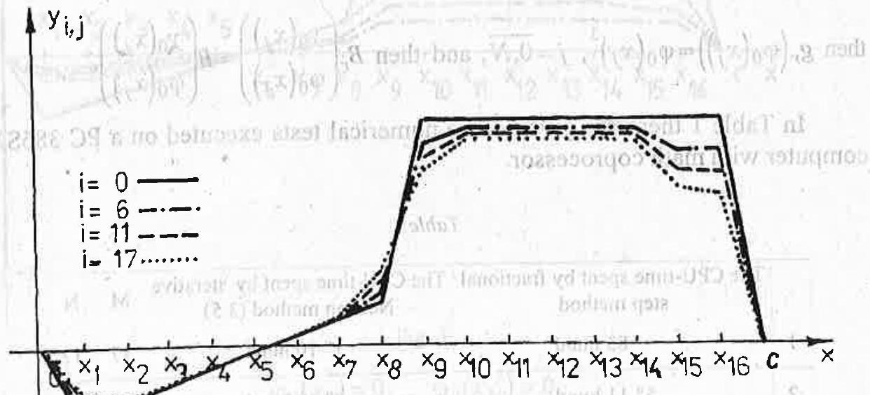
The initial value
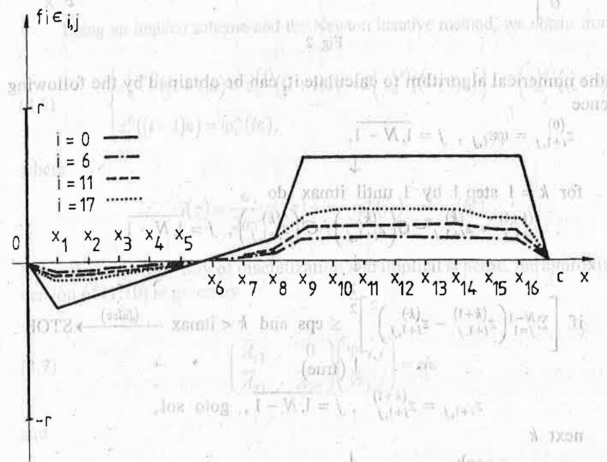
Fig. 3
and the initial value
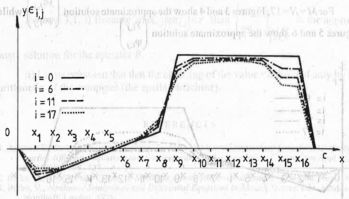
Fig. 4
(see also [10] or [12]).
We observe that
then
In Table 1 there are given some numerical tests executed on a PC 386SX computer with math coprocessor.
We observe that
then
In Table 1 there are given some numerical tests executed on a PC 386SX computer with math coprocessor.
Table 1
| The CPU-time spent by fractional step method | The CPU-time spent by iterative Newton method (3.5) | M | N | |
| 1 | 83 hund | 1" 10 hund | 17 | 17 |
| 2 | 5" 11 hund | 7" 42 hund | 17 | 37 |
| 3 | 8" 89 hund | 11"26 hund | 27 | 37 |
| 4 | 11" 37 hund | 15" 92 hund | 37 | 37 |
| 5 | 14" 94 hund | 47 | 37 |
For
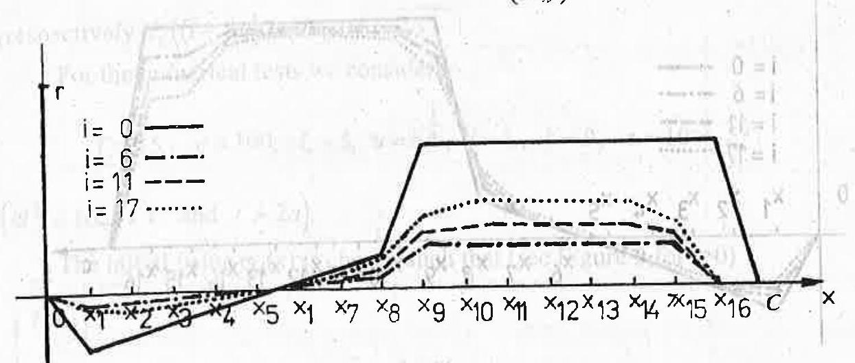
Fig. 5
Fig. 5
Remark 3.1. i) Because
ii) Let us point out that that the choosing of the value
ii) Let us point out that that the choosing of the value
REFERENCES
- Agmon, S., Douglis, A. and Nirenberg, L., Estimates near the boundary for solutions of elliptic partial differential equations satisfying general boundary conditions, Comm. Pure Appl. Math. 12 (1959), 623-727.
- Barbu, V., Analysis and Control of Nonlinear Infinite Dimensional Systems, Academic Press, 1993.
- Barbu, V., Nonlinear Semigroups and Differential Equations in Banach Spaces, Edit. Academiei, Nordhoff, Leyden, 1976.
- Barbu, V., Probleme la limită pentru ecuatii cu derivate partiale, Editura Academiei Romane, Bucureşti, 1993.
- Barbu, V. and Iannelli, M., Approximating some non-linear equations by a Fractional step Scheme, Differential and Integral Equations 1 (1993), 15-26.
- Bates, P. W. and Zheng Songmu, Inertial manifolds and inertial sets for the phase-field equations, in vol. Dynamical Systems, Plenum, (1992), 375-398.
- Brézis, H., Analyse Fonctionnelle. Théorie et Applications. Masson, Paris, 1983.
- Brézis, H., Problèmes unilatéraux, J. Math. Pures. Appl. 51 (1972), 1-168.
- Caginalp, G. An analysis of a phase field model of a free boundary. Arch. Rat. Mech. Anal., 92 (1986), 205-245.
- Caginalp, G. and Nishiura, Y., The existence of travelling waves for phases field equations and convergence to sharp interface models in the singular limit, Quaterly Appl. Math. XLIX 1(1991), 147-162.
- Elliott, C. M. and Zheng, S., Global existence and stability of solutions to the phase field equations, in: Free Boundary Problems, K-H. Hoffinan and J. Sprekels, eds., Int. Ser. of Numerical Math. Vol.95, Birkhäuser Verlag, Basel (1990).
- Fife, C. P., Models for phase separation and their mathematics, nonlinear par. diff eqns. and appl., M. Mimura & T. Nishida, eds., (to appear).
- Morosanu, G., Nonlinear Evolution Equations and Applications, Reidel, Dordrecht, 1988.
- Moroşanu, G., et al. Controlul optimal al suprafetei de solidificare in procesele de turnare continuă a ofelului, Contract nr. 590/115, Etapa II/1993, Capitolul I.
- Pavel, N. H., Differential Equations, Flow Invariance and Applications, Research Notes in Mathematics, 113, Pitnan Advanced Publishing Program (1984).
- Vrabie, I., Compactness Methods for Nonlinear Evolutions. Longman Scientific and Technical, London 1987.
Received 15.09.1995
Department of Mathematics University of Iasi 6000 Iasi Romania
Fig. 6
Copyright (c) 2015 Journal of Numerical Analysis and Approximation Theory

This work is licensed under a Creative Commons Attribution 4.0 International License.


